mls94-complete[1]

l2

r2 θ2

yl1

r1 θ1x

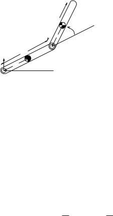
Figure 4.4: Two-link planar manipulator.

2.3Example: Dynamics of a two-link planar robot

To illustrate how Lagrange’s equations apply to a simple robotic system, consider the two-link planar manipulator shown in Figure 4.4. Model each link as a homogeneous rectangular bar with mass mi and moment of inertia tensor

00 Izi

relative to a frame attached at the center of mass of the link and aligned with the principle axes of the bar. Letting vi R3 be the translational velocity of the center of mass for the ith link and ωi R3 be the angular velocity, the kinetic energy of the manipulator is

Since the motion of the manipulator is restricted to the xy plane, kvik is the magnitude of the xy velocity of the center of mass and ωi is a vector

We solve for the kinetic energy in terms of the generalized coordinates by using the kinematics of the mechanism. Let pi = (xi, yi, 0) denote the position of the ith center of mass. Letting r1 and r2 be the distance from the joints to the center of mass for each link, as shown in the figure, we

164

(4.11) The first term in this equation represents the inertial forces due to accel-

eration of the joints, the second represents the Coriolis and centrifugal forces, and the right-hand side is the applied torques.

2.4Newton-Euler equations for a rigid body

Lagrange’s equations provide a very general method for deriving the equations of motion for a mechanical system. However, implicit in the derivation of Lagrange’s equations is the assumption that the configuration space of the system can be parameterized by a subset of Rn, where n is the number of degrees of freedom of the system. For a rigid body with configuration g SE(3), Lagrange’s equations cannot be directly used to determine the equations of motion unless we choose a local parameterization for the configuration space (for example, using Euler angles to parameterize the orientation of the rigid body). Since all parameterizations of SE(3) are singular at some configuration, such a derivation can only hold locally.

In this section, we give a global characterization of the dynamics of a rigid body subject to external forces and torques. We begin by reviewing the standard derivation of the equations of rigid body motion and then examine the dynamics in terms of twists and wrenches.

Let g = (p, R) SE(3) be the configuration of a coordinate frame attached to the center of mass of a rigid body, relative to an inertial frame. Let f represent a force applied at the center of mass, with the coordinates of f specified relative to the inertial frame. The translational

165

equations of motion are given by Newton’s law, which can written in terms of the linear momentum mp˙ as

f = dtd (mp˙).

Since the mass of the rigid body is constant, the translational motion of the center of mass becomes

These equations are independent of the angular motion of the rigid body because we have used the center of mass to represent the position of the body.

Similarly, the equations describing angular motion can be derived independently of the linear motion of the system. Consider the rotational motion of a rigid body about a point, subject to an externally applied torque τ . To derive the equations of motion, we equate the change in angular momentum to the applied torque. The angular momentum relative to an inertial frame is given by I′ω∫ , where

I′ = RIRT

is the instantaneous inertia tensor relative to the inertial frame and ωs is the spatial angular velocity. The angular equations of motion become

τ = dtd (I′ω∫ ) = (RIRT ω∫ ),

where τ R3 is specified relative to the inertial frame. Expanding the right-hand side of this equation, we have

=I′ω˙ ∫ + RR˙ T I′ω∫ + I′RR˙ T ω∫

=I′ω˙ ∫ + ω∫ × I′ω∫ − I′ω∫ × ω∫ ,

where the last equation follows by di erentiating the identity RRT = I and using the definition of ωs. The last term of this equation is zero, and hence the dynamics are given by

Equation (4.13) is called Euler’s equation.

Equations (4.12) and (4.13) describe the dynamics of a rigid body in terms of a force and torque applied at the center of mass of the object. However, the coordinates of the force and torque vectors are not written relative to a body-fixed frame attached at the center of mass, but rather with respect to an inertial frame. Thus the pair (f, τ ) R6 is not the

166

wrench applied to the rigid body, as defined in Chapter 2, since the point of application is not the origin of the inertial coordinate frame. Similarly, the velocity pair (p,˙ ωs) does not correspond to the spatial or body velocity, since p˙ is not the correct expression for the linear velocity term in either body or spatial coordinates.

In order to express the dynamics in terms of twists and wrenches, we rewrite Newton’s equation using the body velocity vb = RT p˙ and body force f b = RT f . Expanding the right-hand side of equation (4.12),

and pre-multiplying by RT , the translational dynamics become

Equation (4.14) is Newton’s law written in body coordinates.

Similarly, we can write Euler’s equation in terms of the body angular velocity ωb = RT ωs and the body torque τ b = RT τ . A straightforward computation shows that

Equation (4.15) is Euler’s equation, written in body coordinates. Note that in body coordinates the inertia tensor is constant and hence we use I instead of I′ = RIRT .

Combining equations (4.14) and (4.15) gives the equations of motion for a rigid body subject to an external wrench F applied at the center of

This equation is called the Newton-Euler equation in body coordinates. It gives a global description of the equations of motion for a rigid body subject to an external wrench. Note that the linear and angular motions are coupled since the linear velocity in body coordinates depends on the current orientation.

It is also possible to write the Newton-Euler equations relative to a spatial coordinate frame. This version is explored in Exercises 4 and 5. Once again the equations for linear and angular motion are coupled, so that the translational motion still depends on the rotational motion. In this book we shall always write the Newton-Euler equations in body coordinates, as in equation (4.16).

167

3Dynamics of Open-Chain Manipulators

We now derive the equations of motion for an open-chain robot manipulator. We shall use the kinematics formulation presented in the previous chapter to write the Lagrangian for the robot in terms of the joint angles and joint velocities. Using this form of the dynamics, we explore several fundamental properties of robot manipulators which are of importance when proving the stability of robot control laws.

3.1The Lagrangian for an open-chain robot

To calculate the kinetic energy of an open-chain robot manipulator with n joints, we sum the kinetic energy of each link. For this we define a coordinate frame, Li, attached to the center of mass of the ith link. Let

represent the configuration of the frame Li relative to the base frame of the robot, S. The body velocity of the center of mass of the ith link is given by

where Jslb i is the body Jacobian corresponding to gsli . Jslb i has the form

is the jth instantaneous joint twist relative to the ith link frame. To streamline notation, we write Jslb i as Ji for the remainder of this section.

The kinetic energy of the ith link is

where Mi is the generalized inertia matrix for the ith link. Now the total kinetic energy can be written as

The matrix M (θ) Rn×n is the manipulator inertia matrix. In terms of the link Jacobians, Ji, the manipulator inertia matrix is defined as

n

X

168

To complete our derivation of the Lagrangian, we must calculate the potential energy of the manipulator. Let hi(θ) be the height of the center of mass of the ith link (height is the component of the position of the center of mass opposite the direction of gravity). The potential energy for the ith link is

Vi(θ) = mighi(θ),

where mi is the mass of the ith link and g is the gravitational constant. The total potential energy is given by the sum of the contributions from each link:

V (θ) = Vi(θ) = mighi(θ).

Combining this with the kinetic energy, we have

3.2Equations of motion for an open-chain manipulator

where M (θ) is the manipulator inertia matrix and V (θ) is the potential energy due to gravity. It will be convenient to express the kinetic energy as a sum,

The equations of motion are given by substituting into Lagrange’s equations,

where we let Υi represent the actuator torque and other nonconservative, generalized forces acting on the ith joint. Using equation (4.20), we have

169

˙

The Mij term can now be expanded in terms of partial derivatives to yield

i = 1, . . . , n.

Equation (4.21) is a second-order di erential equation in terms of the manipulator joint variables. It consists of four pieces: inertial forces, which depend on the acceleration of the joints; centrifugal and Coriolis forces, which are quadratic in the joint velocities; potential forces, of the

form ∂V ; and external forces, Υi.

∂θi

The centrifugal and Coriolis terms arise because of the non-inertial frames which are implicit in the use of generalized coordinates. In the

functions ijk are called the Christo el symbols corresponding to the inertia matrix M (θ).

The external forces can be divided into two components. Let τi repre-

− ˙

sent the applied torque at the joint and define Ni(θ, θ) to be any other forces which act on the ith generalized coordinate, including conservative forces arising from a potential as well as frictional forces. (The reason for the negative sign in the definition of Ni will become apparent in a moment.) As an example, if the manipulator has viscous friction at the joints, then Ni would be defined as

where β is the damping coe cient. Other forces acting on the manipulator, such as forces applied at the end-e ector, can also be included by reflecting them to the joints (via the transpose of the appropriate Jacobian).

170

In order to put the equations of motion back into vector form, we

(4.23) We call the matrix C the Coriolis matrix for the manipulator; the vector

˙

where τ is the vector of actuator torques and N (θ, θ) includes gravity terms and other forces which act at the joints. This is a second-order vector di erential equation for the motion of the manipulator as a function of the applied joint torques. The matrices M and C, which summarize the inertial properties of the manipulator, have some important properties which we shall use in the sequel:

Lemma 4.2. Structural properties of the robot equations of motion

Equation (4.24) satisfies the following properties:

1. M (θ) is symmetric and positive definite.

˙ − n×n

2. M 2C R is a skew-symmetric matrix.

Proof. Positive definiteness of the inertia matrix follows directly from its definition and the fact that the kinetic energy of the manipulator is zero only if the system is at rest. To show property 2, we calculate the

symmetry property depends upon the particular definition of C given in equation (4.23).

171

θ1

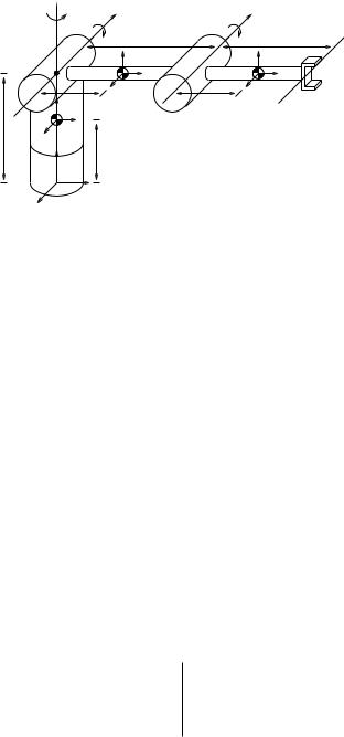
Figure 4.5: Three-link, open-chain manipulator.

Property 2 is often referred to as the passivity property since it implies, among other things, that in the absence of friction the net energy of the robot system is conserved (see Exercise 8). The passivity property is important in the proof of many control laws for robot manipulators.

Example 4.3. Dynamics of a three-link manipulator

To illustrate the formulation presented above, we calculate the dynamics of the three-link manipulator shown in Figure 4.5. The joint twists were computed in Chapter 3 (for the elbow manipulator) and are given by

To each link we attach a frame Li at the center of mass and aligned with principle inertia axes of the link, as shown in the figure:

With this choice of link frames, the link inertia matrices have the general

0Iyi

0 Izi

where mi is the mass of the object and Ixi, Iyi, and Izi are the moments of inertia about the x-, y-, and z-axes of the ith link frame.

172