mls94-complete[1]

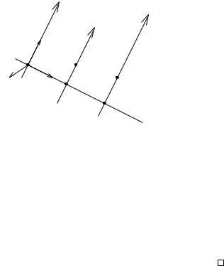
Figure 3.15: End-e ector wrenches which generate no joint torques.

The null space of this matrix is spanned by

hence, workspace torques about the x- and y-axes of the manipulator cannot be applied by the manipulator. For example, twisting the manipulator as shown in Figure 3.15 generates no joint torques and no motion of the manipulator.

4.3Singularities

At a given configuration, the manipulator Jacobian describes the relationship between the instantaneous velocity of the end-e ector and the joint velocities:

s s ˙

Vbt = Jbt(θ)θ.

A singular configuration of a robot manipulator is a configuration at which the manipulator Jacobian drops rank. For a six degree of freedom manipulator in SE(3), the Jacobian fails to be invertible at singular points and hence the manipulator is not able to achieve instantaneous motion in certain directions. Near singular configurations, the size of the joint velocities required to maintain a desired end-e ector velocity in certain directions can be extremely large.

If a manipulator has fewer than six degrees of freedom, a singular configuration corresponds to a configuration in which the number of degrees of freedom of the end-e ector drops. This is again characterized by the manipulator Jacobian dropping rank, i.e., two or more of the columns of Jsts (θ) R6×n become linearly dependent. Since most manipulators

123

are designed for tasks in which all of the degrees of freedom are needed, singular configurations should usually be avoided, if possible.

Singularities also a ect the size of the end-e ector forces that the manipulator can apply. At a singular configuration, some end-e ector wrenches will lie in the null space of the Jacobian transpose. These wrenches can be balanced without applying any joint torques, as the mechanism will generate the opposing wrenches. On the other hand, applying an end-e ector wrench in a singular direction is not possible. Such a wrench could be balanced by any wrench in the singular direction, and hence it can be balanced by the zero wrench. If no other external forces are present, no forces will be generated.

In order to avoid these di culties, it is necessary to identify singular configurations of a manipulator. We concentrate on classifying several common singularities for six degree of freedom manipulators and show how these can be determined by analyzing the geometry of the system. The cases presented here can be extended to consider more general openchain manipulators. For each of the geometric conditions given below, we give a sketch of the proof of singularity. To illustrate some of the di erent ways in which singularities can be analyzed, we use a di erent proof technique for each example.

Example 3.11. Two collinear revolute joints

The Jacobian for a six degree of freedom manipulator is singular if there exist two revolute joints with twists

which satisfy the following conditions:

1.The axes are parallel: ω1 = ±ω2.

2.The axes are collinear: ωi × (q1 − q2) = 0, i = 1, 2.

Proof. In analyzing the singularity of a matrix, we are permitted to preor post-multiply the matrix by a nonsingular matrix of the proper dimensions. Pre-multiplication by a nonsingular matrix can be used to add one row to another or switch two rows, while post-multiplication can be used to perform the same operations on columns.

Assume, without loss of generality, that the columns of the Jacobian which are linearly dependent are the first two columns of J . The Jacobian has the form

124

and we can assume ω1 = ω2 by negating the second column if necessary. Subtracting column 1 from column 2 yields

where the symbol denotes equivalence of two matrices (up to elementary column operations). Using condition 2, the second column is zero, so that J (θ) is singular.

This type of singularity is common in spherical wrist assemblies that are composed of three mutually orthogonal revolute joints whose axes intersect at a point. By rotating the second joint in the wrist, it is possible to align the first and third axes and the manipulator Jacobian becomes singular. In this configuration, rotation about the axis normal to the plane defined by the first and second joints is not possible.

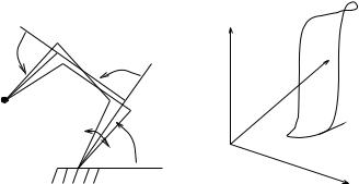
Example 3.12. Three parallel coplanar revolute joint axes

The Jacobian for a six degree of freedom manipulator is singular if there exist three revolute joints which satisfy the following conditions:

1. The axes are parallel: ωi = ±ωj for i, j = 1, 2, 3.

2.The axes are coplanar: there exists a plane with unit normal n such that nT ωi = 0 and

nT (qi − qj ) = 0, i, j = 1, 2, 3.

Proof. Another type of transformation which can be used in analyzing singularities is to change the frame of reference used to express the twists that form the columns of the Jacobian. A change of coordinates a ects twists (and hence the Jacobian) by pre-multiplying by the adjoint matrix corresponding to the change of basis. Since the adjoint is an invertible transformation (Ad−g 1 = Adg−1 ), this does not a ect the singularity of the matrix.

After an initial column permutation, assume J (θ) has the form

Attach a coordinate frame to the point q1 with the z-axis of the frame pointing in the direction of ω1 (see Figure 3.16). Further, choose the frame such that the plane formed by the axes is the yz plane in the new coordinates. Thus, each axis has a point of intersection which lies on the y-axis. Call these points y1(= 0), y2, and y3. Now, with respect to this

125

Figure 3.16: Three coplanar, parallel, revolute twists.

0±y2 ±y3

The first three columns are clearly linearly dependent.

The elbow manipulator exhibits this singularity in its reference configuration (see Figure 3.11).

Example 3.13. Four intersecting revolute joint axes

The Jacobian for a six degree of freedom manipulator is singular if there exist four revolute joint axes that intersect at a point q:

ωi × (qi − q) = 0, i = 1, . . . , 4.

Proof. This example is trivial if we choose a frame whose origin is at the common point of intersection of the four revolute twists. However, we can also show singularity by making use of reciprocal screw systems. Recall from Section 5.3 of Chapter 2 that a wrench is reciprocal to a twist when the inner product between the wrench and the twist is zero (indicating that no work is done by applying the wrench and moving along the twist). Since we are in a 6-dimensional space, if we can show that the dimension of the reciprocal system is su ciently large (three for this example), then we can show singularity of the system of twists. This technique works well when there are a large number of twists and hence the size of the reciprocal system is small.

For this example, we make use of the following fact: every revolute twist is reciprocal to a pure force, in any direction, applied to a point on

126

the axis of the revolute twist. To see this, it su ces to consider a twist and wrench through the origin:

It is left to the reader to verify that this case generalizes appropriately. We can now use this fact to construct the reciprocal system for the

four twists which intersect at a point. Since any pure force through this point corresponds to a reciprocal wrench, it follows that the dimension of the reciprocal system is three and hence the four twists must be singular.

This type of singularity occurs in the inverse elbow manipulator (see Exercise 4) when the final joint axis intersects the shoulder adding a fourth axis as shown.

The singularities given here and in the exercises are by no means exhaustive. However, they do occur frequently and are often easy to determine just by examining the geometry of the manipulator. It is also possible for a manipulator to exhibit di erent types of singularities at a single configuration. In this case, depending on the number and type of the singularities, the manipulator may lose the ability to move in several di erent directions at once. For example, if the arm of the elbow manipulator shown in Figure 3.4 is held vertically over the base, it exhibits all three of the singularities we have just illustrated. However, it still has four degrees of freedom (instead of three) since two of the singularities restrict motion in the same direction.

In addition to singularities of the manipulator Jacobian, a robot can also lose degrees of freedom when the joint variables are constrained to lie in a closed interval. In this case, a loss of freedom of motion can occur when one or more of the joints is at the limit of its travel. At such a configuration, motion past the joint limit is not allowed and the motion of the end-e ector is restricted.

4.4Manipulability

As we saw in the previous section, when a manipulator is at a singular configuration there are directions of movement which require high joint rates and forces. Near a singularity, movement may also be di cult in certain directions. The manipulability of a robot describes its ability to move freely in all directions in the workspace.

Manipulability measures can be divided into two rough classes:

1.The ability to reach a certain position or set of positions

2.The ability to change the position or orientation at a given configuration

127

The first of these measures is directly related to the workspace of a manipulator. Depending on the task, we may want to use the complete, reachable, or dextrous workspaces to characterize the manipulability of a manipulator. The second class of measures concerns the manipulability of a manipulator around a given configuration; that is, it is a local property.

To study local manipulability, we examine the Jacobian of the manipulator, which relates infinitesimal joint motions to infinitesimal workspace motions. Throughout this section we write J for the manipulator Jacobian Jst. Either the spatial or body Jacobian can be used, but the body Jacobian is preferred since the body velocity of the end-e ector is independent of the choice of base frame.

There are many di erent local manipulability measures that have been proposed in the literature and which are useful in di erent situations. We present a small sample of some of the more common measures here. Many of these measures rely on the singular values of J . Recall that for a matrix A Rp×n, the singular values of A are the square roots of the eigenvalues of AT A. We write σ(A) for the set of singular values of A and λ(A) to denote the set of eigenvalues of A. The maximum singular value of a matrix is equal to the induced two-norm of the matrix:

σmax(A) = max kAxk2 = kAk2.

kxk2=1

If a matrix is singular, then at least one of its singular values is zero.

Example 3.14. Minimum singular value of J

µ1(θ) = σmin(J (θ))

The minimum singular value of the Jacobian corresponds to the minimum workspace velocity that can be produced by a unit joint velocity vector. The corresponding eigenvector gives the direction (twist) in which the motion of the end-e ector is most limited. At a singular configuration, the minimum singular value of J is zero.

Example 3.15. Inverse of the condition number of J

µ2(θ) = σmin(J (θ)) σmax(J (θ))

The condition number of a matrix A is defined as the ratio of the maximum singular value of A to the minimum singular value of A. For the Jacobian, the inverse condition number gives a measure of the sensitivity of the magnitude of the end-e ector velocity V to the direction of the

˙

joint velocity vector θ. It provides a normalized measure of the minimum singular value of J . At a singular configuration, the inverse condition number is zero.

128

Example 3.16. Determinant of J

µ3(θ) = det J (θ)

The determinant of the Jacobian measures the volume of the velocity ellipsoid (in the workspace) generated by unit joint velocity vectors. It is important to note that µ3(θ) does not contain information about the condition number of J . In particular, since det J (θ) is the product of

the singular values of J (θ), it can be large even if σmin(J (θ)) is small, by having a large σmax(J (θ)).

These manipulability measures can be used to provide an alternate definition for the dextrous workspace of a manipulator. For any of the measures given above, define the set WD′ as

WD′ is the set of end-e ector configurations for which the manipulator can move infinitesimally in any direction. Note that WD′ is a subset of SE(3), unlike our previous definition (in equation (3.13)) which consisted of the subset of R3 at which the manipulator could achieve any orientation.

Additional manipulability measures are given in the exercises.

5Redundant and Parallel Manipulators

In this section, we briefly consider some other kinematic mechanisms that occur frequently in robotic manipulation. We focus on two particular types of structures—redundant manipulators and parallel manipulators— and indicate how to extend some of the results of this chapter to cover these cases.

5.1Redundant manipulators

In order to perform a given task, a robot must have enough degrees of freedom to accomplish that task. In the analysis presented so far, we have concentrated on the case in which the robot has precisely the required degrees of freedom. A kinematically redundant manipulator has more than the minimal number of degrees of freedom required to complete a set of tasks.

A redundant manipulator can have an infinite number of joint configurations which give the same end-e ector configuration. The extra degrees of freedom present in redundant manipulators can be used to avoid obstacles and kinematic singularities or to optimize the motion of the manipulator relative to a cost function. Additionally, if joint limits are present, redundant manipulators can be used to increase the workspace of the manipulator.

129

The derivation of the forward kinematics of a redundant manipulator is no di erent from the derivation presented in Section 2. Using the product of exponentials formula,

where n is greater than p, the dimension of the workspace (p = 3 for planar manipulators and p = 6 for spatial manipulators). The Jacobian of a redundant manipulator has the form

Jsts (θ) = ξ1 ξ2′ · · · ξn′ ,

where ξi′ is the twist corresponding to the ith joint axis in the current configuration. Jsts Rp×n has more columns than rows.

The inverse kinematics problem for a redundant manipulator is illposed: there may exist infinitely many configurations of the robot which give the desired end-e ector configuration. In fact, if we keep the end- e ector configuration fixed, the robot is still free to move along any trajectory which satisfies

where gd SE(3) is the desired configuration of the end-e ector. The set of all θ which satisfy this equation is called the self-motion manifold for the configuration gd. Di erentiating equation (3.62), we obtain

s ˙ −1

Jst(θ(t))θ = (g˙stgst ) = 0.

Thus, the motions which are allowed must have joint velocities which lie in the null space of the manipulator Jacobian. A motion along the self-motion manifold is called an internal motion.

More generally, given an end-e ector path g(t), we would like to find a corresponding joint trajectory θ(t). Since there may be an infinite number of joint trajectories which give the requisite end-e ector path, additional criteria are used to choose among them. One common solution is to choose the minimum joint velocity which gives the desired workspace velocity. This is achieved by choosing

˙†

θ= Jst(θ)Vst,

where J † = J T (J J T )−1 is the Moore-Penrose generalized inverse of J . The properties of this and other kinematic redundancy resolution algorithms are discussed briefly in Chapter 7.

The manipulator Jacobian can also be used to relate joint torques to end-e ector wrenches for redundant manipulators. Since the links of the manipulator are free to move even when the end-e ector is fixed, a thorough understanding of the relationship between joint forces and end- e ector wrenches requires a study of the dynamics of the manipulator.

130

(x, y)

VN θ1

θ1

Figure 3.17: Self-motion manifold for a redundant planar manipulator.

In particular, the possible existence of internal motions, combined with the inertial coupling between the links, can cause forces to be applied to the end-e ector even if no joint torques are applied. We defer a complete discussion of this situation until Chapter 6, in which we study the dynamics of constrained systems in full detail. Using the results of that chapter, it will be possible to show that when a manipulator is in static equilibrium, the previous relationship,

still holds. This relationship gives the joint torques necessary to produce a given end-e ector wrench when the system is stationary. Either the body or spatial Jacobian can be used, as long as the wrench F is represented appropriately.

Example 3.17. Self-motion manifold for a planar manipulator

Consider the planar manipulator shown in Figure 3.17a. Holding the position of the end-e ector fixed, the system obeys the following kinematic constraints:

l1 cos θ1 + l2 cos(θ1 + θ2) + l3 cos(θ1 + θ2 + θ3) = x l1 sin θ1 + l2 sin(θ1 + θ2) + l3 sin(θ1 + θ2 + θ3) = y.

This is a set of two equations in three variables and hence there exist multiple solutions. A self-motion manifold for this manipulator is shown in Figure 3.17b.

The Jacobian for the mapping p : θ 7→(x, y) is

131

Figure 3.18: A parallel manipulator consisting of three series chains connected to a single end-e ector.

where sijk = sin(θi + θj + θk) and similarly for cijk. The Jacobian has a null space spanned by the vector

− l1l2 sin θ2 + l1l3 sin(θ2 + θ3)

˙

Any velocity θ = αVN is tangent to the self-motion manifold and maintains the position of the end-e ector. One such velocity is shown as an arrow on Figure 3.17b.

5.2Parallel manipulators

A parallel manipulator is one in which two or more series chains connect the end-e ector to the base of the robot. An example is shown in Figure 3.18. Parallel manipulators can o er advantages over open-chain manipulators in terms of rigidity of the mechanism and placement of the actuators. For example, the manipulator in Figure 3.18 can be completely actuated by controlling only the first link in each chain, eliminating the need to place motors at the distal links of the manipulator. Parallel manipulators are also called closed-chain manipulators, since they contain one or more closed kinematic chains.

Structure equation for a parallel mechanism

The forward kinematics for a parallel manipulator are described by equating the end-e ector location specified by each chain. Suppose we have a manipulator with n1 joints in the first chain (including the end-e ector) and n2 joints in the second chain (including the end-e ector). Then, the forward kinematics is described in exponential coordinates as

132