

mls94-complete[1]
.pdf
|
θ2 |
|
joint 2 |
|
|
θ1 |
|
|
joint 1 |
link 2 |
joint 3 (prismatic) |
link 1 |
θ3 |
link 3 |
|
||
|
|
|
|
θ4 |
joint 4 (revolute) |
|
link 4 |
|
|
|
|
Base (link 0) |
|
T |
 S
S
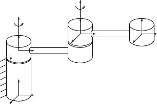
Figure 3.1: Numbering conventions for an AdeptOne robot.
the end-e ector and the joints, and introduces the manipulator Jacobian for a robot. Finally, in Section 5 we extend some of the main results of this chapter to redundant manipulators and parallel mechanisms.
2Forward Kinematics
2.1Problem statement
The forward kinematics of a robot determines the configuration of the end-e ector (the gripper or tool mounted on the end of the robot) given the relative configurations of each pair of adjacent links of the robot. In this section, we restrict ourselves to open-chain manipulators in which the links form a single serial chain and each pair of links is connected either by a revolute joint or a prismatic (sliding) joint. To fix notation, we number the joints from 1 to n, starting at the base, and number the links such that joint i connects links i − 1 and i. Link 0 is taken to be the base of the manipulator and link n is attached rigidly to the end- e ector. Figure 3.1 illustrates our choice of notational conventions for an AdeptOne robot (a type of SCARA manipulator).
The joint space Q of a manipulator consists of all possible values of the joint variables of the robot. This is also the configuration space of
83
the robot, since specifying the joint angles specifies location of all of the links of the robot. For revolute joints, the joint variable is given by an angle θi [0, 2π) with the angle 2π equated to the angle 0. This set of joint angles is naturally associated with a unit circle in the plane, denoted S1, and hence we write θi S1 for revolute joints. We measure all joint angles using a right-handed coordinate system, so that an angle about a directed axis is positive if it represents a clockwise rotation as viewed along the direction of the axis. Prismatic joints are described by a linear displacement θi R along a directed axis, where positive displacement is taken along the direction of the axis.
The joint space Q is the Cartesian product between each of these individual joint spaces. The number of degrees of freedom of an openchain manipulator is equal to the the number of joints in the manipulator. For the four degree of freedom SCARA robot of Figure 3.1, for instance, we have θ = (θ1, θ2, θ3, θ4) S1 × S1 × R × S1 = Q. For manipulators with multiple revolute joints, we use Tp to represent the p-torus, defined to be the Cartesian product of p copies of S1: Tp = S1 × · · · × S1. The joint space of a manipulator with p revolute joints and r prismatic joints is Q = Tp × Rr and has p + r degrees of freedom. In practice, Q may be defined to be a subset of this unrestricted joint space in order to account for joint constraints such as finite displacements and rotations.
We attach two coordinate frames to the manipulator, as illustrated in Figure 3.1. The base frame, S, is attached to a point on the manipulator which is stationary with respect to link 0. Usually, S is attached directly to link 0, although this need not be the case, as we shall see later. (The reason for the use of the letter S instead of B is to avoid confusing the base frame with the body frame, which is ordinarily attached to a moving object.) The tool frame, T , is attached to the end-e ector of the robot, so that the tool frame moves when the joints of the robot move.
The forward kinematics problem can now be formalized. For simplicity, we refer to all joint variables as angles, although both angles and displacements are allowed, depending on the joint type. Given a set of joint angles θ Q, we wish to determine the configuration of the tool frame T relative to the base frame S. The forward kinematics is represented by a mapping gst : Q → SE(3) which describes this relationship. The goal of this section is to show how to explicitly construct gst for a given open-chain robot manipulator and explore the structure of this mapping.
Classically, the forward kinematics map for an open-chain manipulator is constructed by composing the rigid motions due to the individual joints. Consider, for example, the two degree of freedom manipulator shown in Figure 3.2. To compute the configuration of the tool frame T relative to the base frame S, we concatenate the rigid motions between
84
θ2 |
|
θ1 |
|
L2 |
T |
 L1
L1
S
Figure 3.2: A two degree of freedom manipulator.
adjacent frames:
gst(θ1, θ2) = gsl1 (θ1)gl1l2 (θ2)gl2t.
The mapping gst : T2 → SE(3) represents the forward kinematics of the manipulator: it gives the end-e ector configuration as a function of the joint angles.
This procedure is easily extended to any open-chain mechanism. If we define gli−1li (θi) as the transformation between the adjacent link frames,
then the overall kinematics are given by |
|
gst(θ) = gsl1 (θ1)gl1l2 (θ2) · · · gln−1ln (θn)gln t. |
(3.1) |
Equation (3.1) is a general formula for the forward kinematics map of an open-chain manipulator in terms of the relative transformations between adjacent link frames.
2.2The product of exponentials formula
A more geometric description of the kinematics can be obtained by using the fact that motion of the individual joints is generated by a twist associated with the joint axis. Recall that if ξ is a twist, then the rigid motion associated with rotating and translating along the axis of the twist is given by
b
gab(θ) = eξθ gab(0).
If ξ corresponds to a prismatic (infinite pitch) joint, then θ R is the amount of translation; otherwise, θ S1 measures the angle of rotation about the axis.
85
Consider again the two degree of freedom manipulator shown in Figure 3.2. Suppose that we fix the first joint and consider the configuration of the tool frame as a function of θ2 only. This is a simple revolute (zeropitch) screw motion about the axis of the second joint and hence we can write
b
gst(θ2) = eξ2θ2 gst(0),
where ξ2 is the twist corresponding to rotation about the second joint. Next, fix θ2 and move only θ1. By composition, the end-e ector configuration becomes
gst(θ1 |
, θ2) = eb1 |
θ |
1 gst(θ2) = eb1 |
θ |
1 eb2 |
θ |
2 gst(0), |
(3.2) |
|
ξ |
ξ |
ξ |
|
|
where ξ1 is the twist associated with the first joint. Equation (3.2) is an alternative formula for the manipulator forward kinematics. Note that ξ1 and ξ2 are constant twists obtained by evaluating the screw motion for each joint at the θ1 = θ2 = 0 configuration of the manipulator.
The simple form of equation (3.2) appears to rely on moving θ2 first, followed by θ1. This allowed us to represent the joint motions as twists about constant axes. To show that this representation does not depend on the order in which we move the joints, we can derive the forward kinematics by moving θ1 first, and then θ2. In this case,
b
gst(θ1) = eξ1θ1 gst(0)
is the motion due to moving θ1 with θ2 fixed. This motion moves the axis of θ2, and rotation of the second link occurs around a new axis,
ξ2′ = Ad ξ |
θ |
ξ2. |
eb1 |
|
1 |
Using the properties of the matrix exponential (see Exercise 8 in Chapter 2), the rigid body transformation
eb2 |
2 = eb1 |
|
1 |
eb2 |
|
2 |
e−b1 |
|
1 |
ξ′ θ |
ξ |
θ |
|
ξ |
θ |
|
ξ |
θ |
|
describes motion about the new axis. Thus,
gst(θ1 |
, θ2) = eb2 |
|
2 eb1 |
|
1 gst(0) |
|
|
|
|
||||
|
ξ′ θ |
|
ξ |
θ |
|
|
|
e−b1 |
|
1 eb1 |
|
|
|
|
= eb1 |
θ |
1 |
eb2 |
θ |
2 |
θ |
θ |
1 gst(0) |
||||
|
ξ |
|
|
ξ |
|
|
ξ |
ξ |
|
||||
bb
=eξ1θ1 eξ2θ2 gst(0),
as before.
We can generalize this procedure to find the forward kinematics map for an arbitrary open-chain manipulator with n degrees of freedom. Let S be a frame attached to the base of the manipulator and T be a frame
86

attached to the last link of the manipulator. Define the reference configuration of the manipulator to be the configuration of the manipulator corresponding to θ = 0 and let gst(0) represent the rigid body transformation between T and S when the manipulator is in its reference configuration. For each joint, construct a twist ξi which corresponds to the screw motion for the ith joint with all other joint angles held fixed at θj = 0. For a revolute joint, the twist ξi has the form
ξi = |
−ωi × qi , |
|
ωi |
where ωi R3 is a unit vector in the direction of the twist axis and qi R3 is any point on the axis.1 For a prismatic joint,
ξi = |
|
0i |
, |
|
|
v |
|
where vi R3 is a unit vector pointing in the direction of translation. All vectors and points are specified relative to the base coordinate frame
S.
Combining the individual joint motions, the forward kinematics map, gst : Q → SE(3), is given by
gst(θ) = eb1 |
|
1 eb2 |
|
2 · · · eb |
gst(0) |
(3.3) |
ξ |
θ |
ξ |
θ |
ξn θn |
|
|
|
|
|
|
|
|
|
The ξi’s must be numbered sequentially starting from the base, but gst(θ) gives the configuration of the tool frame independently of the order in which the rotations and translations are actually performed. Equation (3.3) is called the product of exponentials formula for the manipulator forward kinematics.
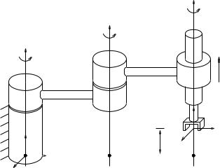
Example 3.1. SCARA forward kinematics
Consider the SCARA manipulator shown in Figure 3.3. It consists of four joints—three revolute and one prismatic (note that we have chosen to order the joints di erently than for the AdeptOne robot in Figure 3.1). We let θ = 0 correspond to the fully extended configuration and attach base and tool frames as shown in the figure.
The transformation between tool and base frames at θ = 0 is given
by |
"I |
l1l0 |
2 |
# . |
gst(0) = |
||||
|
|
0 |
|
|
+l
01
1We choose the convention −ω ×q instead of q ×ω since the former can be correctly interpreted in both the spatial and planar cases (see Exercise 11 in Chapter 2).
87
|
θ3 |
|
|
θ2 |
|
θ1 |
l2 |
|
θ4 |
||
|
||
|
l1 |
z |
T |
|
|
|
l0 |
q1 |
S |
|
|
y |
|
|
q2 |
|
|
|
|
|
|
|
|
q3 |
|
|
|
|
|
|
|
|
|
|
|
|
|
|
|
|
|||||
|
|
|
|
|
|
|
|
|
|
|
|
|
|
|||||
x |
|
|
|
|
|
|
|
|
|
|
|
|
|
|
|
|
|
|
Figure 3.3: SCARA manipulator in its reference configuration. |
||||||||||||||||||
To construct the twists for the revolute joints, note that |
||||||||||||||||||
|
|
|
|
|
|
ω1 = ω2 = ω3 |
= |
0 |
|
|
|
|
|
|
||||
|
|
|
|
|
|
|
|
|
|
|
|
0 |
|
|
|
|
|
|
and we can choose axis points |
|
|
|
|
|
1 |
|
|
|
|
|
|
||||||
|
l1 |
|
q3 = l1 |
+ l2 . |
||||||||||||||
q1 = |
0 |
q2 |
= |
|
||||||||||||||
|
|
0 |
|
|
|
|
0 |
|
|
|
|
|
|
0 |
|
|||
This yields twists |
0 |
|
|
0 |
|
|
|
|
0 |
|||||||||
0 |
|
|
0 |
|
|
= |
|
|
. |
|||||||||
ξ1 = |
ξ2 |
= |
|
ξ3 |
|
0 |
||||||||||||
|
|
|
|
0 |
|
|
|
|
l1 |
|
|
|
|
|
l1+l2 |
|
||
|
|
|
0 |
|
|
|
|
0 |
|
|
|
|
|
0 |
|
|||
|
|
1 |
|
|
1 |
|
|
|
|
1 |
||||||||
|
|
|
|
0 |
|
|
|
|
0 |
|
|
|
|
|
|
0 |
|
|
|
|
|
|
0 |
|
|
|
|
0 |
|
|
|
|
|
|
0 |
|
|
The prismatic joint points in the z direction and has an associated twist
ξ4 |
= |
0 |
= |
0 |
. |
|
|
|
|
0 |
|
|
|
|
|
0 |
|
|
|
v4 |
|
0 |
|
|
|
1 |
|||
|
|
|
0 |
The forward kinematics map of the manipulator has the form
gst(θ) = eb1 |
1 eb2 |
2 eb3 |
3 eb4 |
|
4 gst(0) = |
0 |
1 |
. |
ξ θ |
ξ θ |
ξ θ |
ξ |
θ |
|
R(θ) |
p(θ) |
|
|
|
|
|
88
The individual exponentials are given by |
|
|
|
|
|||||||||
b |
|
|
|
cos θ1 |
− sin θ1 |
0 |
0 |
|
|
|
|||
|
|
|
0 |
|
0 |
|
0 |
1 |
|
|
|||
eξ1 |
θ1 |
= |
sin θ1 |
|
cos θ1 |
0 |
0 |
|
|
||||
|
|
|
|
|
|
|
|
|
|
|
|
|
|
|
|
|
|
|
0 |
|
0 |
|
1 |
0 |
|
|
|
|
|
|
|
|
|
|
|
|
|
||||
b |
|
|
|
cos θ2 |
− sin θ2 |
0 |
|
|
l1 sin θ2 |
|
|||
|
|
|
0 |
|
0 |
|
0 |
|
|
1 |
|||
eξ2 |
θ2 |
= |
sin θ2 |
|
cos θ2 |
0 |
l1(1 − cos θ2) |
||||||
|
|
|
|
|
|
|
|
|
|
|
|
|
|
|
|
|
|
|
0 |
|
0 |
|
1 |
|
|
0 |
|
|
|
|
|
|
|
|
|
|
|
||||
eξ3θ3 = |
sin θ3 |
|
cos θ3 |
0 |
(l1 |
+ l2)(1 − cos θ3) |
|||||||
b |
|
|
|
cos θ3 |
− sin θ3 |
0 |
|
|
(l1 + l2) sin θ3 |
||||
|
|
|
0 |
|
0 |
|
0 |
|
|
1 |
|
||
|
|
|
|
|
|
|
|
|
|
|
|
|
|
|
|
|
|
|
0 |
|
0 |
|
1 |
|
|
0 |
|
|
|
|
|
|
|
|
|
|
|
||||
eξ4θ4 = |
0 1 |
0 0 . |
|
|
|
|
|
||||||
b |
|
|
|
1 |
0 |
0 |
0 |
|
|
|
|
|
|
|
|
0 |
0 |
0 |
1 |
|
|
|
|
|
|||
|
|
|
|
|
|
|
|
|
|
|
|
|
|
|
|
|
|
0 |
0 |
1 |
θ4 |
|
|
|
|
|
|
|
|
|
|
|
|
|
|
|
|
||||
Expanding the terms in the product of exponentials formula yields
|
|
|
|
|
|
|
|
|
|
gst(θ) = |
R(θ) p(θ) |
|
|
|
|
|
|
|
|
|
0 |
1 |
+ θ3) |
cos(θ1 + θ2 |
+ θ3) |
0 |
|
||
R(θ) = |
sin(θ1 |
+ θ2 |
(3.4) |
||||||
|
cos(θ1 |
+ θ2 |
+ θ3) |
− sin(θ1 |
+ θ2 |
+ θ3) |
0 |
|
|
|
|
0 |
|
|
0 |
|
|
1 |
|
p(θ) = |
−l1 cos θ1 |
+ l2 cos(θ1 |
+ θ2) |
. |
|
|
l1 sin θ1 |
− l2 sin(θ1 |
+ θ2) |
||
|
|
|
l0 + θ4 |
|
|
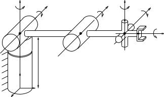
Example 3.2. Elbow manipulator forward kinematics
Consider the elbow manipulator shown in Figure 3.4. The mechanism consists of two intersecting axes at the shoulder, an elbow, and a spherical wrist (modeled as three intersecting axes). The reference configuration (θ = 0) is fully extended, as shown.
The forward kinematics is computed by calculating the individual twist motions for each joint. The transformation between the tool and base frames at θ = 0 is given by
gst(0) = "I |
l1l0 |
2 |
# . |
|
0 |
|
|
+l
|
|
|
|
|
|
|
|
|
|
|
0 |
|
|
1 |
|
|
|
|
|
|
|
|
|
The first two joints have twists |
ξ2 |
= |
|
|
|
1 |
|
|
|
= |
01 |
. |
|||||||||||
ξ1 |
= |
|
0 |
|
|
0 |
« |
= |
0 |
−0 |
|
|
0 « |
||||||||||
|
|
−„ |
0 «×„ |
0 |
|
|
0 |
|
|
|
−„ |
«×„ |
|
|
−l0 |
||||||||
|
|
|
0 |
|
0 |
|
|
|
0 |
|
|
|
|
1 |
|
|
|
0 |
|
|
0 |
|
|
|
|
|
1 |
« |
l |
|
|
|
|
0 |
|
|
|
|
0 |
|
|
« |
l0 |
|
|
0 |
|
|
|
„ 1 |
|
|
|
1 |
|
|
„ 0 |
|
|
||||||||||||
|
|
|
0 |
|
|
|
|
|
|
0 |
|
|
|
|
|
− |
|
|
|
|
|
− |
|
|
|
|
|
|
|
|
|
|
|
|
|
|
|
|
0 |
|
|
|
|
0 |
|
||
89
ξ1 |
|
ξ4 |
ξ2 |
ξ3 |
ξ5 |
l1 |
q2 |
l2 |
q1 |
ξ6 |
|
|
|
T |
l0
S
Figure 3.4: Elbow manipulator.
Note that we have used q1 = (0, 0, l0) for the first twist; we could just as well have used the origin or any other point on the axis of the twist. The other twists are calculated in a similar manner:
ξ3 = |
|
|
1 |
ξ4 = |
0 |
|
|
ξ5 = |
|
|
1 |
|
|
ξ6 = 0 |
. |
||||||||
|
|
0 |
|
|
|
|
|
l1+l2 |
|
|
|
|
0 |
|
|
|
|
|
−l0 |
|
|||
|
|
l |
|
|
|
|
|
|
|
|
|
l |
|
|
|
|
|
|
|||||
|
|
− |
|
0 |
|
|
|
0 |
|
|
|
|
− |
|
0 |
|
|
|
|
0 |
|
||
|
0 |
|
|
1 |
|
|
|
0 |
|
|
|
0 |
|||||||||||
|
|
l1 |
|
|
|
|
0 |
|
|
|
|
l1 |
+l2 |
|
|
|
|
0 |
|
||||
|
|
− |
|
|
|
|
|
|
0 |
|
|
|
|
− |
|
|
|
|
|
|
1 |
|
|
|
|
0 |
|
|
|
|
|
|
|
|
|
|
|
0 |
|
|
|
|
|
|
|
||
The full forward kinematics are |
|
|
|
|
|
|
|
|
|
|
|
|
|
||||||||||
|
|
|
|
|
gst(θ) = eb1 |
1 · · · eb6 6 gst(0) = |
|
0 |
|
1 |
|
|
|
||||||||||
|
|
|
|
|
|
|
ξ |
θ |
|
ξ |
θ |
|
|
R(θ) |
p(θ) |
|
|
|
|||||
|
|
|
|
|
|
|
|
|
|
|
|
|
|
|
|
|
|
|
|
||||
where |
|
|
|
|
|
|
r21 |
|
|
r23 |
|
|
|
|
|
|
|
|
|
|
|
||
|
|
|
|
|
R(θ) = |
r22 |
|
|
|
|
|
|
|
|
|
|
|
||||||
|
|
|
|
|
|
|
r11 |
r12 |
r13 |
|
|
|
|
|
|
|
|
|
|
|
|
||
|
|
|
|
|
p(θ) = |
r31 |
r32 |
r33 |
|
|
|
|
|
|
|
|
, |
|
|
||||
|
|
|
|
|
cos θ1(l1 cos θ2 + l2 cos(θ2 + θ3)) |
|
|
||||||||||||||||
|
|
|
|
|
|
|
− sin θ1 |
(l1 cos θ2 |
+ l2 cos(θ2 |
+ θ3)) |
|
|
|
||||||||||
|
|
|
|
|
|
|
|
l0 − l1 sin θ2 − l2 sin(θ2 + θ3) |
|
|
|
|
|||||||||||
and, using the notation ci |
= cos θi, si |
= sin θi, cij |
= cos(θi + θj ), sij = |
||||||||||||||||||||
90
sin(θi + θj ),
r11 = c6(c1c4 − s1c23s4) + s6(s1s23c5 + s1c23c4s5 + c1s4s5) r12 = −c5(s1c23c4 + c1s4) + s1s23s5
r13 = c6(−c5s1s23 − (c23c4s1 + c1s4)s5) + (c1c4 − c23s1s4)s6
r21 = c6(c4s1 + c1c23s4) − (c1c5s23 + (c1c23c4 − s1s4)s5)s6 r22 = c5(c1c23c4 − s1s4) − c1s23s5
r23 = c6(c1c5s23 + (c1c23c4 − s1s4)s5) + (c4s1 + c1c23s4)s6
r31 = −(c6s23s4) − (c23c5 − c4s23s5)s6 r32 = −(c4c5s23) − c23s5
r33 = c6(c23c5 − c4s23s5) − s23s4s6.
2.3Parameterization of manipulators via twists
Using the product of exponentials formula, the kinematics of a manipulator is completely characterized by the twist coordinates for each of the joints. We now consider some issues related to parameterizing robot motion using twists.
Choice of base frame and reference configuration
In the examples above, we chose the base frame for the manipulator to be at the base of the robot. Other choices of the base frame are possible, and can sometimes lead to simplified calculations. One natural choice is to place the base frame coincident with the tool frame in the reference configuration. That is, we choose a base frame which is fixed relative to the base of the robot and which lines up with the tool frame when θ = 0. This simplifies calculations since gst(0) = I with this choice of base frame and hence
gst(θ) = eb1 |
|
1 · · · eb |
. |
ξ |
θ |
ξn θn |
|
A further degree of freedom in specifying the manipulator kinematics is the choice of the reference configuration for the manipulator. Recall that the reference configuration was the configuration corresponding to setting all of the joint variables to 0. By adding or subtracting a fixed o set from each joint variable, we can define any configuration of the manipulator as the reference configuration. The twist coordinates for the individual joints of a manipulator depend on the choice of reference configuration (as well as base frame) and so the reference configuration is usually chosen such that the kinematic analysis is as simple as possible. For example, a common choice is to define the reference configuration
91

|
θ3 |
|
|
θ2 |
|
θ1 |
l2 |
|
θ4 |
||
|
||
|
l1 |
q1 |
q2 |
|
S, T |
Figure 3.5: SCARA manipulator in its reference configuration, with base frame coincident with tool frame.
such that points on the twist axes for the joints have a simple form, as in all of the examples above.
Example 3.3. SCARA forward kinematics with alternate base frame
Consider the SCARA manipulator with base frame coincident with the tool frame at θ = 0, as shown in Figure 3.5. The twists are now calculated with respect to the new base frame:
ξ1 |
= |
|
|
|
|
0 |
−l1 |
−l2 « |
|
= |
− |
0 |
|
||||
|
|
−„ |
0 «×„ |
|
|
|
10− |
2 |
|||||||||
|
|
|
0 |
|
|
|
|
0 |
|
|
|
|
|
l |
l |
|
|
|
|
1 |
|
„ |
|
« |
0 |
|
|
|
|
0 |
|||||
|
|
|
|
|
|
|
|
|
|
|
|
||||||
|
|
|
|
|
0 |
|
|
|
|
|
|
|
|
0 |
|
||
ξ2 |
|
|
|
|
|
1 |
−l2 « |
|
|
|
|
|
|
1 |
|
||
= |
|
|
0 |
|
= |
0 |
|
|
|||||||||
|
|
−„ |
0 «×„ |
|
|
|
|
−0 |
|
|
|
||||||
|
|
|
0 |
„ |
|
« |
0 |
|
|
|
|
|
|
l2 |
|
|
|
|
|
1 |
1 |
0 |
|
|
|
|
1 |
|
|
||||||
|
|
|
|
|
|
|
|
|
|
|
|
0 |
|
|
|
||
|
|
|
|
|
0 |
|
|
|
|
|
|
|
|
0 |
|
|
|
and similar calculations yield:
ξ3 |
= |
0 |
ξ4 |
= |
0 . |
||||
|
|
|
0 |
|
|
|
|
0 |
|
|
|
|
0 |
|
|
|
|
0 |
|
|
|
1 |
|
|
0 |
||||
|
|
|
0 |
|
|
|
|
1 |
|
|
|
|
0 |
|
|
|
|
0 |
|
92