mls94-complete[1]

Expanding the product of exponentials formula gives

Note that gst(0) = I, which is consistent with the fact that the base and tool frames are coincident at θ = 0. Compare this formula with the kinematics map derived in Example 3.1.

Relationship with Denavit-Hartenberg parameters

Given a base frame S and a tool frame T , the coordinates of the twists corresponding to each joint of a robot manipulator provide a complete parameterization of the kinematics of the manipulator. An alternative parameterization, which is the de facto standard in robotics, is the use of Denavit-Hartenberg parameters [25]. In this section, we discuss the relationships between these two parameterizations and their relative merits.

Denavit-Hartenberg parameters are obtained by applying a set of rules which specify the position and orientation of frames Li attached to each link of the robot and then constructing the homogeneous transformations between frames, denoted gli−1li . By convention, we identify the base frame S with L0. The kinematics of the mechanism can be written as

just as in equation (3.1). Each of the transformations gli−1,li has the form

where the four scalars αi, ai, di, and φi are the parameters for the ith link. For revolute joints, φi corresponds to the joint variable θi, while for prismatic joints, di corresponds to the joint variable θi. DenavitHartenberg parameters are available for standard industrial robots and are used by most commercial robot simulation and programming systems.

It may seem somewhat surprising that only four parameters are needed to specify the relative link displacements, since the twists for each joint have six independent parameters. This is achieved by cleverly choosing

93

the link frames so that certain cancellations occur. In fact, it is possible to give physical interpretations to the various parameters based on the relationships between adjacent link frames. An excellent discussion can be found in Spong and Vidyasagar [110].

There is not a simple one-to-one mapping between the twist coordinates for the joints of a robot manipulator and the Denavit-Hartenberg parameters. This is because the twist coordinates for each joint are specified with respect to a single base frame and hence do not directly represent the relative motions of each link with respect to the previous link. To see this, let ξi−1,i be the twist for the ith link relative to the previous link frame. Then, gli−1li is given by

This is evidently not the same as the product of exponentials formula, though it bears some resemblance to it.

The relationship between the twists ξi and the pairs gli−1li (0) and ξi−1,i can be determined using the adjoint mapping. We first rewrite equation (3.8) as

This formula verifies that the twist ξi is the joint twist for the ith joint in its reference configuration and written relative to the base coordinate frame.

Given the Denavit-Hartenberg parameters for a manipulator, the corresponding twists ξi can be determined by first parameterizing gi−1,i using exponential coordinates, as in equation (3.7), and then applying

94

equation (3.10). However, in almost all instances it is substantially easier to construct the joint twists ξi directly, by writing down the direction of the joint axes and, in the case of revolute joints, choosing a convenient point on each axis. Indeed, one of the most attractive features of the product of exponentials formula is its usage of only two coordinate frames, the base frame S, and the tool frame T . This property, combined with the geometric significance of the twists ξi, make the product of exponentials representation a superior alternative to the use of Denavit-Hartenberg parameters.

2.4Manipulator workspace

The workspace of a manipulator is defined as the set of all end-e ector configurations which can be reached by some choice of joint angles. If Q is the configuration space of a manipulator and gst : Q → SE(3) is the forward kinematics map, then the workspace W is defined as the set

The workspace is used when planning a task for the manipulator to execute; all desired motions of the manipulator must remain within the workspace. We refer to this notion of workspace as the complete workspace of a manipulator.

Characterizing the workspace as a subset of SE(3) is often somewhat di cult to interpret. Instead, one can consider the set of positions (in R3) which can be reached by some choice of joint angles. This set is called the reachable workspace and is defined as

where p(θ) : Q → R3 is the position component of the forward kinematics map gst. The reachable workspace is the volume of R3 which can be reached at some orientation.

Since the reachable workspace does not consider ability to arbitrarily orient the end-e ector, for some tasks it is not a useful measure of the range of a manipulator. The dextrous workspace of a manipulator is the volume of space which can be reached by the manipulator with arbitrary orientation:

WD = {p R3 : R SO(3), θ with gst(θ) = (p, R)} R3. (3.13)

The dextrous workspace is useful in the context of task planning since it allows the orientation of the end-e ector to be ignored when positioning objects in the dextrous workspace.

For a general robot manipulator, the dextrous workspace can be very di cult to calculate. A common feature of industrial manipulators is to

95

θ3

θ2

l3 l2

l1 θ1

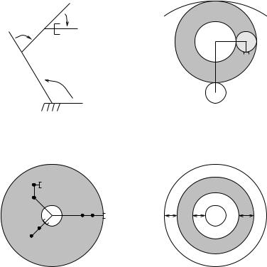
Figure 3.6: Workspace calculations for a planar three-link robot (a). The construction of the workspace is illustrated in (b). The reachable workspace is shown in (c) and the dextrous workspace is shown in (d).

place a spherical wrist at the end of the manipulator, as in the elbow manipulator given in Example 3.2. Recall that a spherical wrist consists of three orthogonal revolute axes which intersect at a point. If the end- e ector frame is placed at the origin of the wrist axes, then the spherical wrist can be used to achieve any orientation at a given end-e ector position. Hence, for a manipulator with a spherical wrist, the dextrous workspace is equal to the reachable workspace, WD = WR. Furthermore, the complete workspace for the end-e ector satisfies W = WR × SO(3). This analysis only holds when the end-e ector frame is placed at the center of the spherical wrist; if an o set is present, the analysis becomes more complex.

Example 3.4. Workspace for a planar three-link robot

Consider the planar manipulator shown in Figure 3.6a. Let g = (x, y, φ)

96

represent the position and orientation of the end-e ector. The forward kinematics of the mechanism can be derived using the product of exponentials formula, but are more easily derived using plane geometry:

We take l1 > l2 > l3, and assume l1 > l2 + l3.

The reachable workspace is calculated by ignoring the orientation of the end-e ector. To generate it, we first take θ1 and θ2 as fixed. The set of reachable points becomes a circle of radius l3 formed by sweeping θ3 through all angles (see Figure 3.6b). We now let θ2 vary through all angles to get an annulus with inner radius l2 − l3 and outer radius l2 + l3 centered at the end of the first link. Finally, we generate the reachable workspace by sweeping the annulus through all values of θ1, to give the reachable workspace. The final construction is shown in Figure 3.6c. WR is an annulus with inner radius l1 − l2 − l3 and outer radius l1 + l2 + l3.

The dextrous workspace for this manipulator is somewhat subtle. Although the manipulator has the planar equivalent of a spherical wrist, the end-e ector frame is not aligned with the center of the wrist. This reduces the size of the dextrous workspace by 2l3 on the inner and outer edges, as shown in Figure 3.6d.

3Inverse Kinematics

We now consider the inverse kinematics problem: given a desired configuration for the tool frame, find joint angles which achieve that configuration. That is, given a forward kinematics map gst : Q → SE(3) and a desired configuration gd SE(3), we would like to solve the equation

for some θ Q. This problem may have multiple solutions, a unique solution, or no solution.

3.1A planar example

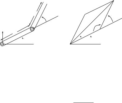
To illustrate some of the issues in inverse kinematics, we first consider the inverse kinematics of the planar two-link manipulator shown in Figure 3.7a. The forward kinematics can be determined using plane geometry:

x = l1 cos θ1 + l2 cos(θ1 + θ2) y = l1 sin θ1 + l2 sin(θ1 + θ2).

97

Figure 3.7: Inverse kinematics of a planar two-link manipulator.

The inverse problem is to solve for θ1 and θ2, given x and y. A standard trick is to solve the problem using polar coordinates, (r, φ), as shown in

If α 6= 0, there are two distinct values of θ2 which give the appropriate radius; the second is referred to as the “flip solution” and is shown as a dashed line in Figure 3.7b. The complete solution is given by solving for φ and using this to determine θ1. This problem must be solved for each possible value of θ2, yielding

where the sign used for β agrees with that used for α.

This planar example illustrates several important features of inverse kinematics problems. In solving an inverse kinematics problem, one first divides the problem into specific subproblems, such as solving for θ2 given r and then using θ1 to rotate the end-e ector to the proper position. Each subproblem may have zero, one, or many solutions depending on the desired end-e ector location. If the configuration is outside of the workspace of the manipulator, then no solution can exist and one of the subproblems must fail to have a solution (consider what happens if r > l1 + l2 in the example above). Multiple solutions occur when the desired configuration is within the workspace but there are multiple joint configurations which all map to the same end-e ector location. If a subproblem generates multiple solutions, then we must complete the solution procedure for all joint angles generated by the subproblem.

98

Traditionally, inverse kinematics solutions are separated into classes: closed-form solutions and numerical solutions. Closed-form solutions, such as the one given above, allow for fast and e cient calculation of the joint angles which give a desired end-e ector configuration. Numerical solutions rely on an interactive procedure to solve equation (3.15). Most industrial manipulators have closed-form solutions. These solutions are obtained in a manner similar to that described above: using geometric and algebraic identities, solve the set of nonlinear, coupled, algebraic equations which define the inverse kinematics problem. An introduction to classical techniques for solving inverse kinematics problems is given in Craig [21].

3.2Paden-Kahan subproblems

Using the product of exponentials formula for the forward kinematics map, it is possible to develop a geometric algorithm to solve the inverse kinematics problem. This method was originally presented by Paden [85] and built on the unpublished work of Kahan [46].

To solve the inverse kinematics problem, we first solve a number of subproblems which occur frequently in inverse solutions for common manipulator designs. One then seeks to reduce the full inverse kinematics problem into appropriate subproblems whose solutions are known. One feature of the subproblems presented here is that they are both geometrically meaningful and numerically stable. Note that this set of subproblems is by no means exhaustive and there may exist manipulators which cannot be solved using these canonical problems. Additional subproblems are explored in the exercises.

For each of the subproblems presented below, we give a statement of the geometric problem to be solved and a detailed solution. On a first reading of this section, it may be di cult to understand the relevance of the specific subproblems presented here. We recommend that the firsttime reader skip the solutions until she sees how the subproblems are used in the examples presented later in this section.

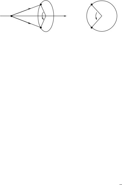
Solution. This problem corresponds to rotating a point p about a given axis ξ until it coincides with a second point q, as shown in Figure 3.8a. Let r be a point on the axis of ξ. Define u = (p − r) to be the vector between r and p, and v = (q − r) the vector between r and q. It follows

b

from equation (3.17) and the fact that exp(ξθ)r = r (since r is on the axis of ξ) that

99

Figure 3.8: Subproblem 1: (a) Rotate p about the axis of ξ until it is coincident with q. (b) The projection of u and v onto the plane normal to the twist axis.

where we have used the fact that u and v are vectors, and hence we have

b

exp(ξθ)u = exp(ωθb )u.

To determine when the problem has a solution, define u′ and v′ to be the projections of u and v onto the plane perpendicular to the axis of ξ. If ω R3 is a unit vector in the direction of the axis of ξ, then

The problem has a solution only if the projections of u and v onto the ω-axis and onto the plane perpendicular to ω have equal lengths. More formally, if we project equation (3.18) onto the span of ω and the null space of ωT , we obtain the necessary conditions

If equation (3.19) is satisfied, then we can find θ by looking only at the projected vectors u′ and v′ as shown in Figure 3.8b. If u′ 6= 0, then we can determine θ using the relationships

If u′ = 0, then there are an infinite number of solutions since, in this case, p = q and both points lie on the axis of rotation.

Subproblem 2. Rotation about two subsequent axes

Let ξ1 and ξ2 be two zero-pitch, unit magnitude twists with intersecting axes and p, q R3 two points. Find θ1 and θ2 such that

100

θ2

q

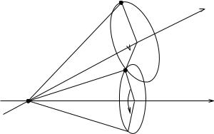
Figure 3.9: Subproblem 2: Rotate p about the axis of ξ2 followed by a rotation around the axis of ξ1 such that the final location of p is coincident with q.

Solution. This problem corresponds to rotating a point p first about the axis of ξ2 by θ2 and then about the axis of ξ1 by θ1, so that the final location of p is coincident with the point q. This motion is depicted in Figure 3.9. If the axes of ξ1 and ξ2 coincide, this problem reduces to Subproblem 1 and any θ1, θ2 such that θ1 + θ2 = θ is a solution, where θ is the solution to Subproblem 1.

If the two axes are not parallel, i.e., ω1 ×ω2 6= 0, then let c be a point such that

In other words, c represents the point to which p is rotated about the axis of ξ2 by θ2. Let r be the point of intersection of the two axes, so that

which implies that

and kuk2 = kzk2 = kvk2. Furthermore, since ω1, ω2, and ω1 × ω2 are linearly independent, we can write

101

and

Substituting equation (3.24) into equation (3.23) gives a system of two equations in two unknowns:

Solving equation (3.25) for γ2 and using kzk2 = kuk2 yields

kuk2 − α2 − β2 − 2αβωT ω2 γ2 = 1 .

This equation may have zero, one, or two real solutions. In the case that a solution exists, we can find z—and hence c—given α, β, and γ.

To find θ1 and θ2, we solve

using Subproblem 1. If there are multiple solutions for c, each of these solutions gives a value for θ1 and θ2. Two solutions exist in the case where the circles in Figure 3.9 intersect at two points, one solution when the circles are tangential, and none when the circles fail to intersect.

Solution. This problem corresponds to rotating a point p about axis ξ until the point is a distance δ from q, as shown in Figure 3.10a. A solution exists if the circle defined by rotating p around ξ intersects the sphere of radius δ centered at q.

To find the explicit solution, we again consider the projection of all points onto the plane perpendicular to ω, the direction of the axis of ξ. Let r be a point on the axis of ξ, and define u = (p − r) and v = (q − r)

102