

mls94-complete[1]
.pdfθ(t)
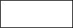
Figure 2.10: Rotational motion of a one degree of freedom manipulator.
Example 2.4. Rotational motion of a one degree of freedom manipulator
Consider the motion of the one degree of freedom manipulator shown in Figure 2.10. Let θ(t) be the angle of rotation about some reference configuration. The trajectory of the manipulator is given by
|
|
|
|
|
|
R(t) = sin θ(t) |
|
cos θ(t) |
0 . |
|
|
|
|
|
|||||
|
|
|
|
|
|
|
|
|
cos θ(t) |
− sin θ(t) 0 |
|
|
|
|
|
||||
The spatial velocity is |
|
0 |
|
|
|
0 |
1 |
|
|
|
|
|
|||||||
|
|
|
|
|
|
|
|
|
|
|
|
|
|||||||
b |
s |
˙ |
T |
|
2−θ˙ sin θ |
−θ˙ cos θ |
03 2 cos θ |
sin θ |
03 |
|
20 |
−θ˙ |
03 |
||||||
|
|
|
4 |
0 |
− |
0 |
05 4 |
|
0 |
0 |
15 40 |
0 05 |
|||||||
ω = RR |
|
= |
|
θ cos θ |
|
θ sin θ |
0 |
|
− sin θ |
cos θ |
0 |
= |
θ |
0 |
0 , |
||||
hence, |
|
|
|
|
|
|
|
ωs = |
0 . |
|
|
|
|
|
|
||||
|
|
|
|
|
|
|
|
|
|
|
|
|
|
|
|||||
|
|
|
|
|
|
|
|
|
|
|
0 |
|
|
|
|
|
|
|
|
The body velocity is |
|
|
|
|
θ˙ |
|
|
|
|
|
|
|
|||||||
|
|
|
|
ωb = RT R˙ = θ˙ |
0 |
0 |
or |
ωb = 0 . |
|
|
|||||||||
|
|
|
|
|
|
|
|
0 |
˙ |
0 |
|
|
|
|
0 |
|
|
|
|
|
|
|
|
b |
|
|
0 |
0 |
0 |
|
|
θ˙ |
|
|
|||||
4.2Rigid body velocity
Let us now consider the general case where gab(t) SE(3) is a oneparameter curve (parameterized by time) representing a trajectory of a rigid body: more specifically, the rigid body motion of the frame B
53
attached to the body, relative to a fixed or inertial frame A. As in the case of rotation, g˙ab(t) by itself is not particularly useful, but the two terms g˙abgab−1 and gab−1g˙ab have some special significance. With
|
|
|
gab(t) = |
0 |
|
|
1 |
|
, |
|
|
|
|
|
|
|
|
|
|
Rab(t) pab(t) |
|
|
|
|
|
||||
we have that |
|
0 |
− 1 |
= |
|
|
|
|
− |
|
|
, |
||
g˙abgab− = |
0 |
0 |
˙ |
0 |
|
˙ |
0 |
|||||||
1 |
˙ |
p˙ab |
T |
T |
|
|
T |
|
|
T |
|
|||
Rab |
Rab |
Rabpab |
|
|
RabRab |
|
RabRabpab + p˙ab |
|
||||||
which has the form of a twist. By analogy to the rotational velocity, we
|
|
|
V s |
|
se(3) as |
|
|
|
|
||
define the spatial velocity bab |
|
s |
|
|
|
R˙ abRT pab + p˙ab |
|
|
|||
V s |
= g˙ |
g−1 |
V s = |
|
vab |
= |
− |
ab |
. |
(2.53) |
|
|
|
ab |
|||||||||
b |
|
ab ab |
|
ωabs |
|
" |
|
|
# |
|
|
ab |
|
ab |
|
|
(R˙ abRT ) |
|
|||||
b s
The spatial velocity Vab can be used to find the velocity of a point in spatial coordinates. The coordinates of a point q attached to the rigid body in spatial coordinates are given by
qa(t) = gab(t)qb.
Di erentiating yields
vqa = q˙a = g˙abqb = g˙abgab−1qa
and thus,
V s q |
a |
= ωs |
q |
a |
+ vs . |
(2.54) |
vqa = bab |
ab × |
|
ab |
|
The interpretation of the components of the spatial velocity of a rigid motion is somewhat unintuitive. The angular component, ωabs , is the instantaneous angular velocity of the body as viewed in the spatial frame. The linear component, vabs , is not the velocity of the origin of the body frame, which is apparent from equation (2.53). Rather, vabs (t) is the velocity of a (possibly imaginary) point on the rigid body which is traveling through the origin of the spatial frame at time t. That is, if one stands at the origin of the spatial frame and measures the instantaneous velocity of a point attached to the rigid body and traveling through the origin at that instant, this is vabs (t).
A somewhat more natural interpretation of the spatial velocity is obtained by using the relationship between twists and screws described in
b s
the previous section. The screw associated with the twist Vab gives the instantaneous axis, pitch, and magnitude of the rigid motion relative to the spatial frame.
54
It is also possible to specify the velocity of a rigid body with respect to the (instantaneous) body frame. We define
Vab = gab− g˙ab = |
|
ab0 |
0 |
Vab = "ωb |
# = "(RT R˙ ab) # |
||||||
|
|
|
|
|
T |
˙ |
|
|
ab |
ab |
p˙ab |
b |
b |
1 |
|
R |
|
Rab |
Rabp˙ab |
b |
ab |
ab |
|
|
|
|
|
|
|
|
|
|
|
|
|
(2.55)
to be the body velocity of a rigid motion gab(t) SE(3). The velocity of the point in the body frame is given by
−1 |
vqa |
= g−1g˙ |
ab |
q |
V b |
(t)q |
. |
vqb = gab |
ab |
|
b = bab |
b |
|
b b
Thus, the action of Vab is to take the body coordinates of a point, qb, and return the velocity of that point written in body coordinates, vqb :
V b q |
b |
= ωb |
q |
b |
+ vb . |
(2.56) |
vqb = bab |
ab × |
|
ab |
|
The interpretation of the body velocity is straightforward: vabb is the velocity of the origin of the body coordinate frame relative to the spatial frame, as viewed in the current body frame. ωabb is the angular velocity of the coordinate frame, also as viewed in the current body frame. Note that the body velocity is not the velocity of the body relative to the body frame; this latter quantity is always zero.
The spatial and body velocity of a rigid motion are related by a similarity transformation. To calculate this relationship, we note that
V s |
= g˙ |
ab |
g−1 |
= g |
ab |
(g−1g˙ |
ab |
)g−1 |
V b |
g−1. |
bab |
|
ab |
|
ab |
ab |
= gab bab |
ab |
Alternatively, we can write
ωabs = Rabωabb
vabs = −ωabs × pab + p˙ab = pab × (Rabωabb ) + Rabvabb .
In either case, we may summarize the calculation as
|
|
|
|
|
b |
|
ab |
# . |
|
s |
vabs |
|
|
Rab |
pabRab |
|
vabb |
|
|
Vab = |
ωabs |
|
= |
0 |
Rab |
|
"ωb |
(2.57) |
The 6 × 6 matrix which transforms twists from one coordinate frame to another is referred to as the adjoint transformation associated with g, written Adg . Thus, given g SE(3) which maps one coordinate system into another, Adg : R6 → R6 is given as
Adg = |
R |
pR |
(2.58) |
|
0 |
b |
|
|
|
R |
|
55
In the calculation that we have just performed, Adg maps body velocity twist coordinates to spatial velocity twist coordinates. Adg is invertible, and its inverse is given by
Adg−1 = |
0 |
−(R RT |
= |
0 |
−RT |
|
= Adg−1 |
|
RT |
T p) RT |
|
RT |
RT p |
|
|
|
|
|
|
|
|
b |
|
(see Exercise 14).
We shall make frequent use of the adjoint transformations throughout the book. The calculations performed above give the following useful characterization of the adjoint associated with a rigid transformation g SE(3):
b 6
Lemma 2.13. If ξ se(3) is a twist with twist coordinates ξ R , then
b −1 6 for any g SE(3), gξg is a twist with twist coordinates Adg ξ R .
It will often be convenient to define velocity without explicit reference to coordinate frames. For a rigid body with configuration g SE(3), we define the spatial velocity as
Vb s = gg˙ −1
and the body velocity as
Vb b = g−1g˙
V s = ωs |
= −(RR˙ T ) |
|
||||||
|
v |
s |
|
|
|
˙ T |
p + p˙ |
|
|
|
|
|
|
RR |
|
||
V b = |
ωb |
= |
"(RT R˙ ) # . |
|
||||
|
|
v |
b |
|
|
RT p˙ |
|
|
|
|
|
|
|
|
|
|
|
(2.59)
(2.60)
The body and spatial velocities are related by the adjoint transformation,
V s = Adg V b. |
(2.61) |
Example 2.5. One degree of freedom manipulator
Consider the one degree of freedom manipulator shown in Figure 2.11. The configuration of the coordinate frame B relative to the fixed frame A is given by
g(t) = |
sin θ(t) |
cos θ(t) |
0 |
l1 |
+ l2 cos θ(t) |
, |
||
|
|
cos θ(t) |
− sin θ(t) |
0 |
−l2 sin θ(t) |
|
|
|
|
0 |
0 |
0 |
|
1 |
|
||
|
|
|
|
|
|
|
|
|
|
|
0 |
0 |
1 |
|
l0 |
|
|
|
|
|
|
|
||||
where we drop all subscripts for simplicity. The spatial velocity of the
rotating rigid body is given by |
|
|
|
|
|
||
V = |
ωs |
ωs |
= (RR˙ |
T ) . |
|||
|
v |
s |
v |
s |
˙ |
T |
p + p˙ |
s |
|
|
= −RR |
||||
56
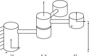
 θ
θ
 B
B
l0
 A
A
|
|
|
|
l1 |
|
l2 |
|
Figure 2.11: Rigid body motion generated by rotation about a fixed axis.
Using the calculation of ωs from the previous example, we have
˙ l1θ
vs = 0 0
0
ωs = 0 .
˙
θ
Note that vs is precisely the velocity of a point attached to the rigid body as it travels through the origin of the A coordinate frame.
The body velocity is
V b = |
ωb |
|
|
ωb = (RT R˙ ) , |
|
|
vb |
|
|
|
vb = RT p˙ |
which gives |
−02 |
|
|
ωb = 0 . |
|
vb = |
˙ |
||||
|
|
l |
θ |
|
0 |
|
0 |
|
θ˙ |
||
The body velocity can be interpreted by imagining the velocity of the origin of the B coordinate frame, as seen in the B coordinates. Thus, the linear velocity is always in the −x direction and the angular velocity is always in the z direction. The magnitude of the linear component of the velocity is dependent on the length of the link connecting the B frame to the joint.
4.3Velocity of a screw motion
In the previous example, we calculated the spatial velocity of a rigid mo-
b
tion generated by a screw action, exp(ξθ). Referring back to Example 2.3
57
in the previous section, we see that the spatial velocity V s in the example
˙
above is identical to ξ when θ = 1. Consider the more general case where
b
gab(θ) = eξθ gab(0)
represents the configuration of coordinate frame B relative to frame A.
b
Using the fact that for a constant twist ξ,
d |
eb |
= ξθe˙ b |
|
dt |
|||
|
ξθ |
b |
ξθ |
(see Exercise 8), the spatial velocity for this rigid body motion is
Vabs = g˙ab(θ)gab−1(θ) |
|
||
b |
b |
b |
|
= ξθe˙ |
ξθ gab(0) |
|
|
b˙
= ξθ.
gab− |
(0)e−b |
1 |
ξθ |
Thus, the spatial velocity corresponding to this motion is precisely the velocity generated by the screw.
The body velocity of a screw motion can be calculated in a similar manner:
|
Vabb |
= gab−1(θ)g˙ab(θ) |
ξθ gab(0) |
|
|
|
|
|
|||||
|
b |
= |
gab−1 |
(0)e−ξθ |
ξθe˙ |
|
|
|
|
|
|||
|
|
|
|
b |
|
b |
|
|
|
|
|
|
|
|
|
= |
g−1 |
(0)ξgab(0) bθ˙ = |
Ad |
1 |
(0) |
ξ |
|
|
θ.˙ |
||
˙ |
b |
|
ab |
|
|
|
|
gab− |
|
|
|
||
|
|
vector in the moving body frame. The di- |
|||||||||||
For θ = 1, Vab is a constant b |
|
|
|
|
|
|
|
|
|
||||
b
rection of the body velocity twist is given by the adjoint transformation generated by the initial configuration of the rigid body, gab−1(0). In particular, if gab(0) = I, i.e., the body frame and spatial frame coincide at
s |
b |
˙ |
θ = 0, then Vab |
= Vab |
= ξθ, where ξ is the constant twist which generates |
the screw motion.
4.4Coordinate transformations
Just as we can compose rigid body transformations to find gac SE(3) given gab, gbc SE(3), it is possible to determine the velocity of one coordinate frame relative to a third given the relative velocities between the first and second and second and third coordinate frames. We state the main results as a set of propositions.
Proposition 2.14. Transformation of spatial velocities
Consider the motion of three coordinate frames, A, B, and C. The following relation exists between their spatial velocities:
Vacs = Vabs + Adgab Vbcs .
58

Proof. The configuration of frame C relative to A is given by
gac = gabgbc.
By definition and the chain rule,
V s |
= g˙ |
ac |
g−1 |
bac |
|
ac |
=(g˙abgbc + gabg˙bc)(gbc−1gab−1)
=g˙abgab−1 + gab(g˙bcgbc−1)gab−1
= V s |
V s g−1 |
, |
bab + gab bbc ab |
|
|
and converting to twist coordinates,
Vacs = Vabs + Adgab Vbcs .
Proposition 2.15. Transformation of body velocities
Consider motion of three coordinate frames, A, B, and C. The following relation exists between their relative body velocities:
Vacb = Adgbc−1 Vabb + Vbcb .
Proof. Application of the chain rule, as above.
Propositions 2.14 and 2.15 are used to transform the velocity of a rigid body between di erent coordinate frames. Often, two of the coordinate frames are stationary with respect to each other and the velocity relationships can be simplified. As an example, if A and B are two inertial frames which are fixed relative to each other, then the spatial velocity of a frame C satisfies
V s |
= Ad |
gab |
V s . |
(2.62) |
ac |
|
bc |
|
The corresponding relationship for body velocities is
Vacb = Vbcb , |
(2.63) |
since the body velocity is independent of the inertial frame with respect to which it is measured.
The transformation rules given by Propositions 2.14 and 2.15 can also be applied to constant twists, such as those used to model revolute and prismatic joints. If ξ is a twist which represents the motion of a screw and we move the screw by applying a rigid body motion g SE(3), the new twist can be obtained using equation (2.62). We interpret g as a fixed rigid motion and equate ξ with a spatial velocity vector. In this case, g˙ = 0 and hence
ξ′ = Ad |
g |
ξ |
or |
b |
b |
(2.64) |
|
ξ′ = gξg−1. |
|||||
59
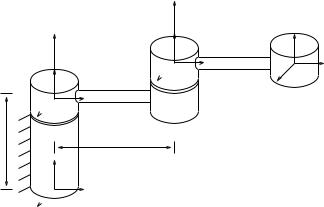
 θ2
θ2
 θ1
θ1
 C
C
 B
B
l0
l1
 A
A
Figure 2.12: Two degree of freedom manipulator.
This formula is of tremendous importance in the chapters to come, where we will need to keep track of the di erent twist axes corresponding to the joints of a robot when they are moved.
Example 2.6. Velocity of a two-link mechanism
Consider the two degree of freedom manipulator shown in Figure 2.12. We wish to find the velocity of frame C relative to A, given the joint
˙ |
˙ |
R. Since each motion is a screw motion, we write |
velocities θ1 |
, θ2 |
Vab = |
ωab |
θ˙1 |
s |
vab |
|
Vbc = |
ωbc |
θ˙2 |
s |
vbc |
|
We also calculate Adgab :
|
|
00
vab = 0 |
ωab = 0 , |
|||
vbc = |
0 |
|
ωbc = |
1 |
0 |
0 . |
|||
|
l1 |
|
0 |
|
|
|
|
|
|
|
0 |
|
|
1 |
|
" |
0 |
|
|
ab |
|
# |
|
|
|
|
|
Rab |
|
|
0 |
|
Rab . |
|
|
|
|
Adgab = |
|
|
0 |
|
|
|
|||
|
|
l0 |
|
|
|
|||||
|
|
|
|
|
R |
|
|
|
|
|
Using Proposition 2.14, |
|
0 |
θ1 + |
|
θ2. |
|||||
Vac = Vab + Adgab Vbc = |
0 |
|||||||||
|
|
|
|
0 |
|
|
|
l1 cos θ1 |
|
|
s |
s |
s |
|
0 |
|
˙ |
|
l1 sin θ1 |
|
˙ |
0 |
0 |
|||||||||
|
|
|
1 |
|
1 |
|
||||
|
|
|
|
0 |
|
|
|
0 |
|
|
Note that the velocity consists of two components, one from each of the joints, and that they add together linearly.
60
A few other identities between body and spatial velocities will prove useful in subsequent chapters. We give them here in the form of a lemma. Their proof is left as an exercise.
Lemma 2.16. Rigid body velocity identities
Using the notation given above for the velocity of one coordinate frame relative to another, the following relationships hold:
Vabb = −Vbas
Vabb = − Adgba Vbab .
5Wrenches and Reciprocal Screws
In this section we consider forces and moments acting on rigid bodies and use this to introduce the notion of screw systems and reciprocal screws.
5.1Wrenches
A generalized force acting on a rigid body consists of a linear component (pure force) and an angular component (pure moment) acting at a point. We can represent this generalized force as a vector in R6:
f |
f R3 |
linear component |
F = τ |
|
rotational component |
τ R3 |
We will refer to a force/moment pair as a wrench.
The values of the wrench vector F R6 depend on the coordinate frame in which the force and moment are represented. If B is a coordinate frame attached to a rigid body, then we write Fb = (fb, τb) for a wrench applied at the origin of B, with fb and τb specified with respect to the B coordinate frame.
Wrenches combine naturally with twists to define instantaneous work. Consider the motion of a rigid body parameterized by gab(t), where A is an inertial frame and B is a frame attached to the rigid body. Let Vabb R6 represent the instantaneous body velocity of the rigid body and let Fb represent an applied wrench. Both of these quantities are represented relative to the B coordinate frame and their dot product is the infinitesimal work:
δW = Vabb · Fb = (v · f + ω · τ ).
The net work generated by applying the wrench Fb through a twist Vabb over a time interval [t1, t2] is given by
Z t2
W = Vabb · Fb dt.
t1
61
|
|
x |
|
|
F |
z |
B |
|
y |
||
z |
|
||
|
|
||
C |
y |
|
|
|
|
|
x
A |
Figure 2.13: Transformation of wrenches between coordinate frames.
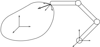
Two wrenches are said to be equivalent if they generate the same work for every possible rigid body motion. Equivalent wrenches can be used to rewrite a given wrench in terms of a wrench applied at a di erent point (and with respect to a di erent coordinate frame). An example of this is shown in Figure 2.13: given the wrench Fb applied at the origin of contact coordinate frame B, we wish to determine the equivalent wrench applied at the origin of the object coordinate frame C. In order to compute the equivalent wrench, we use the instantaneous work performed by the wrench as the body undergoes an arbitrary rigid motion. Let gbc = (pbc, Rbc) be the configuration of frame C relative to B. By equating the instantaneous work done by the wrench Fb and the wrench Fc over an arbitrary interval of time, we have that
Vacb · Fc = Vabb · Fb = Adgbc Vacb T Fb = Vacb · AdTgbc Fb,
and since V b |
is free, |
|
ac |
Fc = AdgTbc Fb. |
|
|
(2.65) |
Equation (2.65) transforms a wrench applied at the origin of the B frame into an equivalent wrench applied at the origin of the C frame. The components of Fc are specified relative to the C coordinate frame. Expanding equation (2.65),
fc |
= " |
RbcT |
0 |
# |
fb |
, |
(2.66) |
|
τc |
RT pbc |
RT |
τb |
|||||
|
|
bc |
b |
bc |
|
|
|
|
|
− |
|
|
|
|
|
|
|
we see that the adjoint transformation rotates the force and torque vectors from the B frame into the C frame and includes an additional torque of the form −pbc × fb, which is the torque generated by applying a force fb
at a distance −pbc.
It is also possible to represent a wrench with respect to a coordinate frame which is not inside the rigid body. Consider for example the co-
62