mls94-complete[1]

Table 4.1: Summary of the basic theorem of Lyapunov.

− ˙

3. If V (x, t) is locally positive definite and decrescent, and V (x, t) is locally positive definite, then the origin of the system is uniformly locally asymptotically stable.

− ˙

4. If V (x, t) is positive definite and decrescent, and V (x, t) is positive definite, then the origin of the system is globally uniformly asymptotically stable.

The conditions in the theorem are summarized in Table 4.1.

Theorem 4.4 gives su cient conditions for the stability of the origin of a system. It does not, however, give a prescription for determining the Lyapunov function V (x, t). Since the theorem only gives su cient conditions, the search for a Lyapunov function establishing stability of an equilibrium point could be arduous. However, it is a remarkable fact that the converse of Theorem 4.4 also exists: if an equilibrium point is stable, then there exists a function V (x, t) satisfying the conditions of the theorem. However, the utility of this and other converse theorems is limited by the lack of a computable technique for generating Lyapunov functions.

Theorem 4.4 also stops short of giving explicit rates of convergence of solutions to the equilibrium. It may be modified to do so in the case of exponentially stable equilibria.

Theorem 4.5. Exponential stability theorem

x = 0 is an exponentially stable equilibrium point of x˙ = f (x, t) if and only if there exists an ǫ > 0 and a function V (x, t) which satisfies

α1kxk2 ≤ V (x, t) ≤ α2kxk2

for some positive constants α1, α2, α3, α4, and kxk ≤ ǫ.

183

The rate of convergence for a system satisfying the conditions of Theorem 4.5 can be determined from the proof of the theorem [102]. It can be shown that

are bounds in equation (4.34). The equilibrium point x = 0 is globally exponentially stable if the bounds in Theorem 4.5 hold for all x.

4.3The indirect method of Lyapunov

The indirect method of Lyapunov uses the linearization of a system to determine the local stability of the original system. Consider the system

with f (0, t) = 0 for all t ≥ 0. Define

∂f (x, t)

A(t) = (4.38)

∂x x=0

to be the Jacobian matrix of f (x, t) with respect to x, evaluated at the origin. It follows that for each fixed t, the remainder

f1(x, t) = f (x, t) − A(t)x

approaches zero as x approaches zero. However, the remainder may not approach zero uniformly. For this to be true, we require the stronger condition that

If equation (4.39) holds, then the system

is referred to as the (uniform) linearization of equation (4.31) about the origin. When the linearization exists, its stability determines the local stability of the original nonlinear equation.

Theorem 4.6. Stability by linearization

Consider the system (4.37) and assume

Further, let A(·) defined in equation (4.38) be bounded. If 0 is a uniformly asymptotically stable equilibrium point of (4.40) then it is a locally uniformly asymptotically stable equilibrium point of (4.37).

184

K

M

B

q

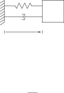
Figure 4.8: Damped harmonic oscillator.

The preceding theorem requires uniform asymptotic stability of the linearized system to prove uniform asymptotic stability of the nonlinear system. Counterexamples to the theorem exist if the linearized system is not uniformly asymptotically stable.

If the system (4.37) is time-invariant, then the indirect method says that if the eigenvalues of

∂f (x) A =

∂x x=0

are in the open left half complex plane, then the origin is asymptotically stable.

This theorem proves that global uniform asymptotic stability of the linearization implies local uniform asymptotic stability of the original nonlinear system. The estimates provided by the proof of the theorem can be used to give a (conservative) bound on the domain of attraction of the origin. Systematic techniques for estimating the bounds on the regions of attraction of equilibrium points of nonlinear systems is an important area of research and involves searching for the “best” Lyapunov functions.

4.4Examples

We now illustrate the use of the stability theorems given above on a few examples.

Example 4.5. Linear harmonic oscillator

Consider a damped harmonic oscillator, as shown in Figure 4.8. The dynamics of the system are given by the equation

185

where M , B, and K are all positive quantities. As a state space equation we rewrite equation (4.41) as

Define x = (q, q˙) as the state of the system.

Since this system is a linear system, we can determine stability by examining the poles of the system. The Jacobian matrix for the system

which has a characteristic equation

λ2 + (B/M )λ + (K/M ) = 0.

which always have negative real parts, and hence the system is (globally) exponentially stable.

We now try to apply Lyapunov’s direct method to determine exponential stability. The “obvious” Lyapunov function to use in this context is the energy of the system,

Taking the derivative of V along trajectories of the system (4.41) gives

− ˙

The function V is quadratic but not locally positive definite, since it does not depend on q, and hence we cannot conclude exponential stability. It is still possible to conclude asymptotic stability using Lasalle’s invariance principle (described in the next section), but this is obviously conservative since we already know that the system is exponentially stable.

The reason that Lyapunov’s direct method fails is illustrated in Figure 4.9a, which shows the flow of the system superimposed with the level sets of the Lyapunov function. The level sets of the Lyapunov function become tangent to the flow when q˙ = 0, and hence it is not a valid Lyapunov function for determining exponential stability.

To fix this problem, we skew the level sets slightly, so that the flow of the system crosses the level surfaces transversely. Define

186

Figure 4.9: Flow of damped harmonic oscillator. The dashed lines are the level sets of the Lyapunov function defined by (a) the total energy and (b) a skewed modification of the energy.

where ǫ is a small positive constant such that V is still positive definite. The derivative of the Lyapunov function becomes

˙

The function V can be made negative definite for ǫ chosen su ciently small (see Exercise 11) and hence we can conclude exponential stability. The level sets of this Lyapunov function are shown in Figure 4.9b.

This same technique is used in the stability proofs for the robot control laws contained in the next section.

Example 4.6. Nonlinear spring mass system with damper

Consider a mechanical system consisting of a unit mass attached to a nonlinear spring with a velocity-dependent damper. If x1 stands for the position of the mass and x2 its velocity, then the equations describing the system are:

x˙ 1 = x2

(4.45)

x˙ 2 = −f (x2) − g(x1).

Here f and g are smooth functions modeling the friction in the damper and restoring force of the spring, respectively. We will assume that f, g are both passive; that is,

σf (σ) ≥ 0 σ [−σ0, σ0] σg(σ) ≥ 0 σ [−σ0, σ0]

187

and equality is only achieved when σ = 0. The candidate for the Lya-

The passivity of g guarantees that V (x) is a locally positive definite function. A short calculation verifies that

This establishes the stability, but not the asymptotic stability of the origin. Actually, the origin is asymptotically stable, but this needs Lasalle’s principle, which is discussed in the next section.

4.5Lasalle’s invariance principle

Lasalle’s theorem enables one to conclude asymptotic stability of an equi-

− ˙

librium point even when V (x, t) is not locally positive definite. However, it applies only to autonomous or periodic systems. We will deal with the autonomous case and begin by introducing a few more definitions. We denote the solution trajectories of the autonomous system

as s(t, x0, t0), which is the solution of equation (4.46) at time t starting from x0 at t0.

Definition 4.7. ω limit set

The set S Rn is the ω limit set of a trajectory s(·, x0, t0) if for every y S, there exists a strictly increasing sequence of times tn such that

s(tn, x0, t0) → y

as tn → ∞.

Definition 4.8. Invariant set

The set M Rn is said to be an (positively) invariant set if for all y M and t0 ≥ 0, we have

s(t, y, t0) M t ≥ t0.

It may be proved that the ω limit set of every trajectory is closed and invariant. We may now state Lasalle’s principle.

Theorem 4.7. Lasalle’s principle

{ ˙ }

S = x Ωc : V (x) = 0 .

188

As t → ∞, the trajectory tends to the largest invariant set inside S; i.e., its ω limit set is contained inside the largest invariant set in S. In particular, if S contains no invariant sets other than x = 0, then 0 is asymptotically stable.

A global version of the preceding theorem may also be stated. An application of Lasalle’s principle is as follows:

Example 4.7. Nonlinear spring mass system with damper

Consider the same example as in equation (4.45), where we saw that with

we obtained

˙ −

V (x) = x2f (x2).

Choosing c = min(V (−σ0, 0), V (σ0, 0)) so as to apply Lasalle’s principle, we see that

˙ ≤ { ≤ }

V (x) 0 for x Ωc := x : V (x) c .

As a consequence of Lasalle’s principle, the trajectory enters the largest

∩{ ˙ } ∩{ }

invariant set in Ωc x1, x2 : V = 0 = Ωc x1, 0 . To obtain the largest invariant set in this region, note that

x2(t) ≡ 0 = x1(t) ≡ x10 = x˙ 2(t) = 0 = −f (0) − g(x10), where x10 is some constant. Consequently, we have that

g(x10) = 0 = x10 = 0.

∩ { ˙ }

Thus, the largest invariant set inside Ωc x1, x2 : V = 0 is the origin and, by Lasalle’s principle, the origin is locally asymptotically stable.

There is a version of Lasalle’s theorem which holds for periodic systems as well. However, there are no significant generalizations for nonperiodic systems and this restricts the utility of Lasalle’s principle in applications.

5Position Control and Trajectory Tracking

In this section, we consider the position control problem for robot manipulators: given a desired trajectory, how should the joint torques be chosen so that the manipulator follows that trajectory. We would like to choose a control strategy which is robust with respect to initial condition errors, sensor noise, and modeling errors. We ignore the problems of actuator dynamics, and assume that we can command arbitrary torques which are exerted at the joints.

189

5.1Problem description

We are given a description of the dynamics of a robot manipulator in the form of the equation

where θ Rn is the set of configuration variables for the robot and τ Rn denotes the torques applied at the joints. We are also given a joint trajectory θd(·) which we wish to track. For simplicity, we assume that θd is specified for all time and that it is at least twice di erentiable.

Since both θ and θd satisfy the same di erential equation and have the same initial conditions, it follows from the uniqueness of the solutions of di erential equations that θ(t) = θd(t) for all t ≥ 0. This an example of an open-loop control law: the current state of the robot is not used in choosing the control inputs.

Unfortunately, this strategy is not very robust. If θ(0) 6= θd(0), then the open-loop control law will never correct for this error. This is clearly undesirable, since we almost never know the current position of a robot exactly. Furthermore, we have no guarantee that if our starting configuration is near the desired initial configuration that the trajectory of the robot will stay near the desired trajectory for all time. For this reason, we introduce feedback into our control law. This feedback must be chosen such that the actual robot trajectory converges to the desired trajectory. In particular, if our trajectory is a single setpoint, the closed-loop system should be asymptotically stable about the desired setpoint.

There are several approaches for designing stable robot control laws. Using the structural properties of robot dynamics, we will be able to prove stability of these control laws for all robots having those properties. Hence, we do not need to design control laws for a specific robot; as long as we show that stability of a particular control algorithm requires only those properties given in Lemma 4.2 on page 171, then our control law will work for general open-chain robot manipulators. Of course, the performance of a given control law depends heavily on the particular manipulator, and hence the control laws presented here should only be used as a starting point for synthesizing a feedback compensator.

5.2Computed torque

Consider the following refinement of the open-loop control law presented above: given the current position and velocity of the manipulator, cancel

190

all nonlinearities and apply exactly the torque needed to overcome the inertia of the actuator,

¨ ˙ ˙ ˙

τ = M (θ)θd + C(θ, θ)θ + N (θ, θ).

Substituting this control law into the dynamic equations of the manipulator, we see that

¨ ¨

M (θ)θ = M (θ)θd,

Hence, if the initial position and velocity of the manipulator matches the desired position and velocity, the manipulator will follow the desired trajectory. As before, this control law will not correct for any initial condition errors which are present.

The tracking properties of the control law can be improved by adding state feedback. The linearity of equation (4.48) suggests the following control law:

where e = θ − θd, and Kv and Kp are constant gain matrices. When substituted into equation (4.47), the error dynamics can be written as:

M (θ) (¨e + Kv e˙ + Kpe) = 0.

Since M (θ) is always positive definite, we have

This is a linear di erential equation which governs the error between the actual and desired trajectories. Equation (4.49) is called the computed torque control law.

The computed torque control law consists of two components. We can write equation (4.49) as

The term τ is the feedforward component. It provides the amount of torque necessary to drive the system along its nominal path. The term τfb is the feedback component. It provides correction torques to reduce any errors in the trajectory of the manipulator.

Since the error equation (4.50) is linear, it is easy to choose Kv and Kp so that the overall system is stable and e → 0 exponentially as t → ∞.

191

Moreover, we can choose Kv and Kp such that we get independent exponentially stable systems (by choosing Kp and Kv diagonal). The following proposition gives one set of conditions under which the computed torque control law (4.49) results in exponential tracking.

Proposition 4.8. Stability of the computed torque control law

If Kp, Kv Rn×n are positive definite, symmetric matrices, then the control law (4.49) applied to the system (4.47) results in exponential trajectory tracking.

Proof. The error dynamics can be written as a first-order linear system:

It follows that if λ = 0 then v = 0, and hence λ = 0 is not an eigenvalue of A. Further, if λ 6= 0, then v2 = 0 implies that v1 = 0. Thus, v1, v2 6= 0 and we may assume without loss of generality that kv1k = 1. Using this, we write

λ2 = v1 λ2v1 = v1 λv2

= v1 (−Kpv1 − Kv v2) = −v1 Kpv1 − λv1 Kv v1,

where denotes complex conjugate transpose. Since α = v1 Kpv1 > 0 and β = v1 Kv v1 > 0, we have

λ2 + αλ + β = 0 α, β > 0

and hence the real part of λ is negative.

The power of the computed torque control law is that it converts a nonlinear dynamical system into a linear one, allowing the use of any of a number of linear control synthesis tools. This is an example of a more general technique known as feedback linearization, where a nonlinear system is rendered linear via full-state nonlinear feedback. One disadvantage of using feedback linearization is that it can be demanding (in terms of computation time and input magnitudes) to use feedback to globally convert a nonlinear system into a single linear system. For robot manipulators, unboundedness of the inputs is rarely a problem since the inertia matrix of the system is bounded and hence the control torques which must be exerted always remain bounded. In addition, experimental results show that the computed torque controller has very good performance characteristics and it is becoming increasingly popular.

192