mls94-complete[1]

Figure 5.13: Force-closure grasps for an equilateral triangle. The lightly shaded region corresponds to the set of all force-closure grasps and the dark square (and corresponding darkened regions on the triangle) indicates maximally independent regions of contact.

Given any two edges, we can represent these inequalities on a graph, by drawing the lines which correspond to the inequalities becoming identically zero. Figure 5.13 gives an example of such a graph.

This graph gives a complete description of the force-closure grasps between any two edges. By enumerating all pairs of edges, we can generate all possible force-closure grasps for the object. There are many methods which might be used to choose among the grasps. One is to assign a quality measure to a grasp and choose the grasp which maximizes this quality measure and is also force-closure. Another possibility is to choose a grasp such that it is maximally distant from the edges of the force-closure region. Such a grasp is equivalent to choosing maximal independent regions of contact on each edge. That is, we can attempt to find regions on each edge such that if either contact is within the respective region, the grasp is force-closure. Such a region corresponds to a square in the force-closure grasp.

The algorithm presented above can be extended to the spatial case using the following variant of Theorem 5.6:

Theorem 5.7. Spatial antipodal grasps [82]

A spatial grasp with two soft-finger contacts is force-closure if and only if the line connecting the contact point lies inside both friction cones.

It is also possible to extend the algorithm sketched above to work for objects with curved surfaces. In this case, the constraints become nonlinear functions of the contact locations (suitably parameterized). However, the algorithm can still be applied if there is a way to find the

233

zeros of the given expressions.

5Grasp Constraints

In the previous sections, we analyzed the grasp kinematics ignoring the kinematics of the fingers. That is, we assumed that forces could be applied at contact points irrespective of how those forces were generated. In this section, we extend our analysis to include the kinematics and statics of the robotic fingers.

We shall view a robot hand grasping an object as a kinematically constrained system. In correspondence with the preceding sections, we assume that the contact locations are fixed on the object. In this case, the constraints between the object and a finger can be formulated by requiring that certain velocities are equal. For example, at a given contact point, the velocity of the fingertip and the velocity of the contact point (on the object) must agree in the direction normal to the surface. For simplicity, we assume throughout the remainder of this section that all contacts are either point contacts with friction or soft-finger contacts. This justifies our assumption that the contact location is fixed; the more general case is considered in the next section.

5.1Finger kinematics

In Chapter 3 we derived the forward kinematics for an open-chain manipulator using the product of exponentials formula. Recall that the spatial velocity of the end-e ector of the robot can be written as

s s ˙

Vst = Jst(θ)θ,

where Jsts (θ) Rp×n is the spatial Jacobian of the forward kinematics function. The twist Vsts is the generalized velocity of the tool frame, written with respect to a fixed base frame. The body velocity of the tool frame is given by

It represents the instantaneous velocity of the tool frame, written in tool coordinates.

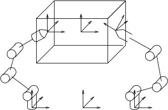
We model a robot hand as a collection of robots (fingers) attached to a common base (palm). For each finger in the hand, attach a frame Si to the base of the finger and a frame Fi to the fingertip at the point of contact, as shown in Figure 5.14. Note that the frame Fi moves with the fingertip, while the frame Ci, also located at the contact point,

moves with the object. Let J s be the Jacobian for Fi relative to the

si fi

fixed frame Si so that

234

Figure 5.14: Grasp coordinate frames.

where θfi Rni is the vector of joint angles for the ith finger.

The grasping constraint for a finger gives the directions in which motion is not allowed. Relative to the contact frame Ci, these constraints can be written as constraints on the velocity of the finger frame Fi. For example, a frictionless point contact restricts the velocities of the finger and the object such that the relative velocity between these two frames is zero in the direction normal to the surface. By convention, this is the z- axis direction in the contact frame, and hence we can write the constraint

as

0 0 1 0 0 0 Vfbi ci = 0.

wrench basis for a frictionless point contact.

In general, the directions in which motion is constrained are precisely those in which forces can be exerted. Hence, for a contact with wrench

Equation (5.9) restricts the relative velocity between the finger and the object to be perpendicular to the directions in which forces can be applied.

We can now proceed to write equation (5.9) in terms of a set of known quantities. We perform all computations using body velocities, and hence we temporarily drop the superscript b. Using the velocity relations in Chapter 2 Section 4, we can write Vfi ci as

Vpfi is the velocity of the fingertip relative to the palm frame. Since the finger base frames are fixed relative to the palm frame, it follows that

We can write Vpci by adding the velocity between the palm and object to the velocity between the object and contact. Since the contact frame is fixed relative to the object frame (by the fixed contact assumption), we have

Substituting equations (5.11) and (5.12) into equation (5.10) gives

Vfi ci = − Ad−gpc1i Adgpfi Vsi fi + Ad−goc1i Vpo.

We can now substitute this into the constraint equation and use the finger kinematics to yield

This equation represents the ith contact constraint in terms the finger joint angles θ and the object configuration gpo.

The contact constraint can be simplified by making use of the adjoint equation

Making this substitution, the constraint for the ith finger becomes

Stacking equation (5.13) for each finger, we can write the constraint in matrix form. Let k be the number of fingers, ni the number of degrees of freedom for the ith finger, and set n = n1 + · · · + nk. Define the hand Jacobian as the matrix Jh(θ, xo) : Rn → Rm given by

236

where xo := gpo is the configuration of the object and θ is the vector of all finger joint angles. Equation (5.15) is the fundamental grasping constraint; it relates velocities of the fingers to the velocity of the object. The quantities in the constraint plus a description of the grasp friction cone provide all of the necessary information for modeling a fixed contact grasp.

Although we have derived the grasp constraint in a very mechanical fashion, it is possible to interpret equation (5.15) in a simple and meaningful way. Equation (5.15) equates the velocity of the object and the velocity of the fingertip at the point of contact between the two. Since motion in some directions may be allowed (for example, rotation about the contact point), we only constrain those directions specified by the columns of Bci . Equation (5.15) is merely a restatement of equation (5.9) written in a more useful form.

The quantities Jh, G, and F C completely characterize the properties of a set of fingers grasping an object. This motivates the following definition.

Definition 5.4. Representation of a multifingered grasp

A multifingered grasp is described by the hand Jacobian Jh(θ, xo) : Rn → Rm, the grasp map G : Rm → Rp, and the friction cone F C Rm which satisfies the properties in Definition 5.1.

Formally, we distinguish between a grasp, which includes specification only of the object and the contact locations, and a multifingered grasp, which includes a description of the finger kinematics. When the usage is clear from context, we use the term grasp.

5.2Properties of a multifingered grasp

We are now in a position to study the mathematical properties of the grasp constraint in equation (5.15) and interpret them. In the beginning of this chapter, we saw that the force-closure properties of a grasp are characterized by the grasp map G and the friction cone F C. In studying force-closure, we assumed that all allowable contact forces could be applied by the fingers; we can now detail under what conditions this is true and what happens when this condition fails.

A fundamental property of a multifingered grasp is the ability of the robot fingers to accommodate an object motion. If a set of fingers can accommodate any motion of the object without losing contact, we say that such a grasp is manipulable:

Definition 5.5. Manipulable grasp

A multifingered grasp is manipulable at a configuration (θ, xo) if for any

The following proposition follows from the definition.

237

Figure 5.15: Diagram of relationships for a multifingered grasp. The contact force must satisfy fc F C for these relationships to hold.

Proposition 5.8. Characterization of all manipulable grasps

A grasp is manipulable at a configuration (θ, xo) if and only if

R(GT ) R(Jh(θ, xo)).

Manipulability does not require that the matrix Jh be injective (one- to-one); there may be many finger motions which accommodate a given object motion. This can happen precisely in the case where Jh is full (row) rank with more columns than rows (n > m), and hence has a

˙ N

non-trivial null space. Any joint velocities θN (Jh) result in no

˙

motion of the contacts; we call θN an internal motion. Internal motions can be added to a given finger velocity without changing the velocity of the grasped object and so the finger-object system becomes a redundant manipulator. Note that this kinematic redundancy may appear even if none of the individual fingers are redundant, due to the Bci terms in the definition of the hand Jacobian. These have the e ect of masking out joint velocities in directions which do not violate the contact constraints, and hence allowing internal motions in those directions.

Equation (5.15) describes the velocity relationships between the object and fingers. We will also make use of the force relationships. As described in Section 2, the grasp map characterizes the relationship between contact forces and object wrenches:

Fo = Gfc.

The contact forces can be related to the joint torques by using the transpose of the hand Jacobian:

(this follows by equating the work done by the joints and contacts). As in our derivation of the grasp map, the contact forces must lie in the friction

238

Table 5.4: Grasp properties.

cone F C in order to avoid slipping. The complete set of relationships between the velocities and forces in a multifingered grasp are summarized in Figure 5.15.

As in Chapter 3, some care must be taken in interpreting equation (5.16) in the case that Jh Rm×n is not square. If the grasp is manipulable and force-closure, then it follows that Jh is surjective onto the range of GT . In this case, we can always exert a given contact force, but the joint torques required may not be unique. If internal motions are present, the dynamics of the manipulator must be taken into account. This is discussed more fully in the next chapter.

If a grasp is not manipulable, then it may not be possible to exert arbitrary contact forces. In this case, JhT will have a non-trivial null space and hence there may exist contact forces fc which give τ = 0 in equation (5.16). This is completely analogous to the case in an open-chain manipulator with fewer joint degrees of freedom than the dimension of the workspace. In particular, we call contact forces which lie in the null space of JhT structurally dependent forces, since they generate forces in the mechanism that cannot be determined without more information about the elastic properties of the mechanism.

As we have seen above, the properties of a grasp can be completely described by the grasp map G, the hand Jacobian Jh, and the friction cone F C. These properties of a grasp are summarized in Table 5.4. Note that force-closure and manipulability are separate properties. It is possible for a grasp to be force-closure but not manipulable, manipulable and not force-closure, or neither force-closure or manipulable. A few of these possibilities are illustrated in Figure 5.16.

239

Figure 5.16: Some grasps illustrating manipulability and force-closure properties.

5.3Example: Two SCARA fingers grasping a box

As an example of how these calculations proceed, consider the grasp shown in Figure 5.17. In this example, two SCARA fingers are used to grasp a box. Assume that the contact points are located at pci = (0, ±r, 0) with respect to the object frame of reference, and that each contact is modeled as a soft-finger contact.

The majority of the quantities needed to describe the grasping constraint have been previously computed. The grasp map was derived in Example 5.2:

0 +r 0 0 −r 0 0 0

using the contact frames shown in Figure 5.5. The wrench basis for each finger was given by

For simplicity, we take the length of the fingertips as l3 = 0 and hence the contact occurs at the usual SCARA end-e ector location. In this case, the Jacobian is that given in Example 3.8:

If l3 6= 0, then we must recompute the Jacobian to include the additional displacement (see Exercise 11).

from the spatial frame into the contact frame for a given finger. We can

240

Figure 5.17: Two-fingered grasp using SCARA robots.

Since the transformations goci and gsi p are constant, we can write

Note that only Ad−gpo1 depends on xo = gpo, the current configuration of the object, and the other transformations are constant matrices.

To construct the grasp constraint, we compose the matrices given above in the appropriate fashion. In full generality, the contact constraints are quite complex and the calculations are more suited for automated rather than manual computation. We therefore restrict ourselves to analyzing the grasp constraints for the object configuration shown in Figure 5.17. That is, we set

and hence Ad−1 becomes a constant matrix. Rather than compute it

gsi ci

in pieces, we use the transformations gsi ci , which can be written down by inspection:

241

Finally, we calculate Jh:

(for the particular configuration shown in Figure 5.17).

We can now evaluate the properties of the grasp. From Example 5.2 we have that the grasp is force-closure (this does not depend on the fingers which actually exert the forces). However, the grasp is not manipulable, since rotation of the object about the y-axis yields

The grasp contains internal motions which are in the vector space spanned

at the configuration shown. These motions correspond to rotating the last revolute joint of each finger, resulting in a rotation of the fingertip about contact point. In the more general case where l3 6= 0 and the hand is in an arbitrary configuration, the internal motion still exists but all three revolute joints will have nonzero instantaneous velocities.

6Rolling Contact Kinematics

Most real-world grasping situations involve moving rather than fixed contacts. Human fingers and many robotic fingers are actually surfaces, and manipulation of an object by a set of fingers involves rolling of the fingers along the object surface. In this section, we derive the kinematic equations for one object rolling against another and extend the grasping

242