θ
d
ψ
l
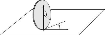
Figure 7.5: A simple hopping robot.
appendages moving in space, where angular momentum is conserved, or a diver or gymnast in mid-air maneuvers.
In the sequel, we will give a description of several nonholonomic systems. The proof of their nonholonomy (that is the impossibility of finding functions of the configuration variables which are “integrals” of the constraints) is deferred to Section 4.
Example 7.2. Hopping robot in flight
As our first example, we consider the dynamics of a hopping robot in the flight phase, as shown in Figure 7.5. This robot consists of a body with an actuated leg that can rotate and extend; the “constraint” on the system is conservation of angular momentum.
The configuration q = (ψ, l, θ) consists of the leg angle, the leg extension, and the body angle of the robot. We denote the moment of inertia of the body by I and concentrate the mass of the leg, m, at the foot. The upper leg length is taken to be d, with l representing the extension of the leg past this point. The total angular momentum of the robot is given by
˙ |
2 ˙ |
˙ |
(7.11) |
Iθ |
+ m(l + d) (θ |
+ ψ). |
Assume that the angular momentum of the robot is initially zero. Equa-
˙ ˙ ˙
tion (7.11) is a single Pfa an constraint in the three velocities ψ, l, and θ. Thus, the associated control system has two inputs—three configuration variables minus one constraint. As a basis for the 2-dimensional right null space of the constraint, we choose one vector field corresponding to controlling the leg angle ψ, and the other corresponding to controlling
 ψ2
ψ2
m
r
θ
l
ψ1
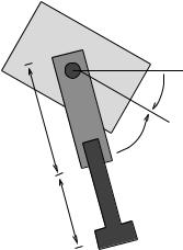
Figure 7.6: A simplified model of a planar space robot.
|
|
˙ |
|
|
˙ |
. Then, we have |
the leg extension l; i.e., set ψ = u1 |
and l = u2 |
g1(q) = |
|
0 |
2 |
|
g2 |
(q) = |
1 |
|
|
|
1 |
|
|
|
|
0 |
|
|
|
|
|
|
|
|
− |
m(l+d) |
|
|
|
|
|
|
|
|
|
|
0 |
|
|
I+m(l+d)2 |
|
|
|
and the equivalent control system is given by q˙ = g1(q)u1 + g2(q)u2.
Example 7.3. Planar space robot
Figure 7.6 shows a simplified model of a planar robot consisting of two arms connected to a central body via revolute joints. If the robot is free floating, then the law of conservation of angular momentum implies that moving the arms causes the central body to rotate. In the case that the angular momentum is zero, this conservation law can be viewed as a Pfa an constraint on the system.
Let M and I represent the mass and inertia of the central body and let m represent the mass of the arms, which we take to be concentrated at the tips. The revolute joints are located a distance r from the middle of the central body and the links attached to these joints have length l. We let (x1, y1) and (x2, y2) represent the position of the ends of each of the arms (in terms of θ, ψ1, and ψ2). Assuming that the body is free floating in space and that friction is negligible, we can derive the constraints arising from conservation of angular momentum.
Let θ be the angle of the central body with respect to the horizontal, ψ1 and ψ2 the angles of the left arm and right arms with respect to the central body, and p R2 the location of a point on the central body (say the center of mass). The kinetic energy of the system has the form
|
|
|
|
|
|
|
|
|
|
|
|
|
|
|
|
|
|
|
1 |
(M + 2m)kp˙k |
2 |
|
1 |
˙2 |
|
|
1 |
|
2 |
2 |
1 |
2 |
2 |
K = |
|
|
+ |
|
Iθ |
+ |
|
|
m(x˙ |
1 |
+ y˙1 ) + |
|
m(x˙ 2 |
+ y˙2 ) |
2 |
|
2 |
2 |
2 |
= 2 (M + 2m) p˙ |
2 + 2 |
ψ˙ |
2 |
|
T |
a12 |
a22 |
a23 |
ψ˙2 , |
|
|
|
|
|
|
˙ |
|
|
a11 |
a12 |
a13 |
˙ |
|
|
1 |
|
|
|
1 |
ψ1 |
|
|
|
ψ1 |
|
|
k k |
|
|
θ˙ |
a13 |
|
a33 θ˙ |
|
|
|
|
|
a23 |
where aij can be calculated as
a11 = a22 = ml2 a12 = 0
a13 = ml2 + mr cos ψ1 a23 = ml2 + mr cos ψ2
a33 = I + 2ml2 + 2mr2 + 2mrl cos ψ1 + 2mrl cos ψ2.
Note that the kinetic energy of the system is independent of the variable θ. It therefore follows from Lagrange’s equations that in the absence of
external forces, |
|
|
|
d ∂L |
|
∂L |
|
|
|
|
|
|
|
|
|
|
|
|
|
|
|
= |
|
= 0. |
|
|
|
|
|
|
|
˙ |
|
|
|
|
|
|
dt ∂θ |
|
∂θ |
|
Thus the quantity |
∂L˙ is a constant of the motion. This is precisely the |
|
∂θ |
|
|
|
|
|
|
|
|
|
|
angular momentum, µ, of the system: |
|
|
|
∂L |
|
|
|
|
˙ |
|
˙ |
˙ |
|
µ = |
˙ |
|
= a13 |
ψ1 |
+ a23ψ2 |
+ a33θ. |
|
|
∂θ |
|
|
|
|
|
|
|
|
If the initial angular momentum is zero, then conservation of angular momentum ensures that the angular momentum stays zero, giving the following constraint equation
˙ |
˙ |
˙ |
(7.12) |
a13(ψ)ψ1 |
+ a23(ψ)ψ2 |
+ a33(ψ)θ = 0. |
Since the variables that are actuated are the hinge angles of the left
|
|
|
|
˙ |
|
˙ |
. Using these in |
and right arm, we choose as inputs u1 = ψ1 and u2 |
= ψ2 |
equation (7.12) and setting q = (ψ1 |
, ψ2, θ), we get |
|
|
|
q˙ = g1(q)u1 + g2(q)u2 |
|
|
|
where |
|
a13 |
|
g2(q) = |
a23 . |
|
g1(q) = |
|
|
|
1 |
|
|
0 |
|
|
|
|
0 |
|
|
1 |
|
|
|
−a33 |
−a33 |
|
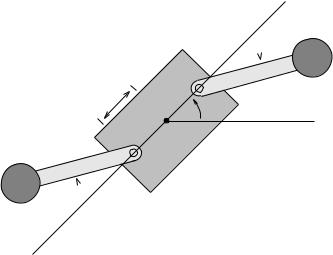
Figure 7.7: Disk rolling on a plane.
Example 7.4. Disk rolling on a plane
Consider the motion of a thin flat disk rolling on a plane shown in Figure 7.7. The configuration space of the system is parameterized by the xy location of the contact point of the disk with the plane, the angle θ that the disk makes with the horizontal line, and the angle φ of a fixed line on the disk with respect to the vertical axis. We assume that the disk rolls without slipping. As a consequence we have that
− ˙
x˙ ρ cos θ φ = 0
− ˙
y˙ ρ sin θ φ = 0,
where ρ > 0 is the radius of the disk. Writing these equations in the form of Pfa an constraints with q = (x, y, θ, φ) we have
|
0 |
1 |
0 −ρ sin θ |
|
|
|
1 |
0 |
0 |
−ρ cos θ |
q˙ = 0. |
|
˙ |
|
|
|
|
|
˙ |
, the rate of turning |
Choosing θ = u1 |
, the rate of rolling, and φ = u2 |
about the vertical axis, we have the associated control system: |
|
q˙ = ρ sin θ u1 |
+ 0 u2. |
(7.13) |
|
|
|
ρ cos θ |
|
0 |
|
|
|
0 |
|
1 |
|
|
|
|
|
|
|
|
|
|
|
|
|
|
|
|
|
10
Example 7.5. Kinematic car
Consider a simple kinematic model for an automobile with front and rear tires, as shown in Figure 7.8. The rear tires are aligned with the car, while the front tires are allowed to spin about the vertical axes. To simplify the derivation, we model the front and rear pairs of wheels as single wheels at the midpoints of the axles. The constraints on the system arise by allowing the wheels to roll and spin, but not slip.
Let (x, y, θ, φ) denote the configuration of the car, parameterized by the xy location of the rear wheel(s), the angle of the car body with
336
φ
l
y
θ
 x
x
Figure 7.8: Kinematic model of an automobile.
respect to the horizontal, θ, and the steering angle with respect to the car body, φ. The constraints for the front and rear wheels are formed by setting the sideways velocity of the wheels to zero. In particular, the velocity of the back wheels perpendicular to their direction is sin θx˙ − cos θy˙ and the velocity of the front wheels perpendicular to the direction
− − ˙
they are pointing is sin(θ +φ)x˙ cos(θ +φ)y˙ lθ cos φ, so that the Pfa an constraints on the automobile are:
− − ˙ sin(θ + φ)x˙ cos(θ + φ)y˙ l cos φ θ = 0
sin θ x˙ − cos θ y˙ = 0.
Converting this to a control system with the inputs chosen as the driving velocity u1 and the steering velocity u2 gives
y˙ |
|
= |
|
1sin θ |
u1 |
+ |
0 u2. |
(7.14) |
|
x˙ |
|
l |
cos θ |
|
|
0 |
|
|
˙ |
|
|
0 |
|
1 |
|
φ |
|
|
|
|
|
|
|
|
|
|
˙ |
|
|
|
|
|
|
|
|
|
|
|
θ |
|
|
|
|
tan φ |
|
|
0 |
|
|
For this choice of vector fields, u1 corresponds to the forward velocity of the rear wheels of the car and u2 corresponds to the velocity of the angle of the steering wheel.
Example 7.6. Fingertip rolling on an object
Let us analyze the motion of a curved fingertip over a curved object. As we discussed in Section 6 of Chapter 5, we parameterize the object surface by αo R2, the fingertip surface by αf R2, and the angle of contact by ψ S1, giving a 5-dimensional configuration space. The kinematic
equations of contact are given by |
|
|
− |
|
|
vy |
|
|
f |
ωx |
|
|
|
α˙ f = M −1(Kf + K˜o)−1 |
|
−ωy |
|
|
K˜o |
vx |
|
o |
|
ωx |
|
|
|
vy |
α˙ o = M −1Rψ (Kf + K˜o)−1 |
−ωy |
|
|
+ Kf |
vx |
(7.15) |
˙
ψ = ωz + Tf Mf α˙ f + ToMoα˙ o.
The rolling constraint is obtained by setting the sliding velocity and the velocity of rotation about the contact normal to zero:
Substituting (7.16) into equation (7.15) yields the following constraints:
Mf α˙ f − Rψ Moα˙ o = 0 |
(7.17) |
˙ |
|
Tf Mf α˙ f + ToMoα˙ o − ψ = 0. |
|
If we set q = (αf , αo, ψ) R5, then the foregoing set of three constraints is of the form
ωi(q)q˙ = 0 i = 1, 2, 3.
To obtain a control system associated with these constraints, we let u1 = ωx and u2 = ωy in the kinematic equations for rolling contact. After rearranging the results, we have
|
|
|
o− |
|
ψ |
|
|
1 |
|
0 |
|
|
|
|
T |
Mf−1 |
|
|
|
|
|
|
|
|
|
|
+ T R |
|
|
|
|
q˙ = |
|
M |
|
1R |
|
ψ |
(Kf + K˜o)−1 |
0 |
u1 + |
−1 |
u2 |
. |
(7.18) |
|
f |
|
o |
|
|
|
|
|
|
|
|
We now specialize the example to the case that the object is flat and the fingertip is a sphere of radius one. The curvature forms, metric tensors, and torsions for the fingertip and the object have been derived in Example 5.7 and are reproduced here for convenience:
Ko = |
0 |
0 |
Kf = |
0 |
1 |
|
|
|
0 |
0 |
|
1 |
0 |
|
|
Mo = |
0 |
1 |
Mf = |
0 |
cos q1 |
|
|
1 |
0 |
|
1 |
0 |
|
|
To = 0 |
0 |
Tf = 0 |
− tan q1 |
. |
Substituting the above results into (7.17) gives
0 |
cos q1 |
−sin q5 |
cos q5 |
0 q˙ = 0. |
1 |
0 |
cos q5 |
sin q5 |
0 |
0 |
sin q1 |
0 |
0 |
1 |

In this case, the formula (7.18) gives, with the inputs being the rates of rolling about the two tangential directions,
q˙2 |
|
|
sec q1 |
|
|
|
|
0 |
|
|
|
|
|
q˙1 |
|
|
|
0 |
|
|
|
|
−1 |
|
|
u2. |
|
q˙3 |
|
= |
|
−cos q5 |
u1 |
+ |
−sin q |
5 |
5 |
(7.19) |
|
4 |
|
|
|
|
5 |
|
|
|
0 |
|
|
|
q˙ |
|
|
−tan q |
|
|
|
|
|
|
|
|
|
q˙ |
|
|
|
sin q |
1 |
|
|
|
cos q |
|
|
|
5 |
|
|
|
|
|
|
|
|
|
|
|
− |
|
|
|
|
|
|
|
|
|
4Structure of Nonholonomic Systems
We return to the problem of motion planning for systems satisfying linear velocity constraints of the form
ωi(q)q˙ = 0 i = 1, . . . , k.
In Section 2 we showed how the problem of finding feasible trajectories in the configuration space could be dualized to one of finding trajectories of the control system
q˙ = g1(q)u1 + · · · + gm(q)um, |
(7.20) |
with m = n − k and ωi(q)gj (q) = 0. From the controllability rank condition, it follows that one can find a trajectory joining an arbitrary starting point and end point if the rank of the Lie algebra generated by g1, . . . , gm is n. If q 6= Tq Rn and in addition q has a constant rank n − p which is less than n, then it follows from Frobenius’ theorem that there exist functions hi(q) = ci, i = 1, . . . , p such that
ωi(q)q˙ = 0 i = 1, . . . , k |
hj (q) = cj |
j = 1, . . . , p. |
Consider this a little further: since the dimension of |
|
is greater than |
|
or equal to the dimension of Δ, it follows that p ≤ k. Thus, the number of functions whose level sets are tangential to the given distribution are fewer than the dimension of the distribution. The process of converting from the given constraints, specified as a codistribution, to an equivalent control system and then integrating the involutive closure of this distribution may seem to be convoluted. It is indeed possible to deal directly with a given codistribution and to find the maximal integrable codistribution contained within it, but this involves methods of exterior di erential systems which are beyond the scope of this book. Of course, in the event that = Tq Rn for all q, then p = 0, i.e., there are no nontrivial functions which integrate the given constraints. In this case the distribution is said to be completely nonholonomic, as was noted earlier.
In this section, we will try to make precise some notation that we will use in dealing with nonholonomic systems and apply it to the examples
that we considered in Section 3. Some additional machinery to study the growth of the controllability Lie algebra is discussed at the end of this section.
4.1Classification of nonholonomic distributions
The complexity of the motion planning problem is related to the order of Lie brackets in its controllability Lie algebra. Here we develop some concepts which allow us to classify nonholonomic systems. Let = span{g1, . . . , gm} be the distribution associated with the control
system (7.20). Define |
1 = |
and |
|
|
|
|
|
i = |
i−1 + [Δ1, |
i−1], |
|
|
where |
i−1] = span{[g, h] : g |
1, h |
i−1}. |
|
[Δ1, |
|
It is clear that i |
|
i+1. The chain of the distributions |
i is defined |
as the filtration associated with the distribution |
= 1. |
Each i is |
defined to be spanned by the input vector fields plus the vector fields formed by taking up to i −1 Lie brackets of the generators, i.e., elements
of |
1. The Jacobi identity |
(see Proposition 7.1, page 325) implies that |
[Δi, |
j ] [Δ1, i+j−1] |
|
i+j . |
The proof of this fact is left as an |
exercise. |
|
|
|
|
A filtration is said to be regular in a neighborhood U of q0 if |
|
rank |
i(q) = rank |
i(q0) |
q U. |
We say the control system (7.20) is regular if the corresponding filtration
is regular. If a filtration is regular, then at each step of its construction, |
i |
either gains dimension or |
i+1 = |
i, so that the construction terminates. |
If rank |
i+1 = rank i, then |
i is involutive and hence i+j = i |
for |
all j ≥ 0. |
Clearly, rank |
i ≤ n and hence if a filtration is regular, then |
there exists an integer κ < n such that i = κ for all i ≥ κ.
Definition 7.2. Degree of nonholonomy
Consider a regular filtration { i} associated with a distribution smallest integer κ such that the rank of κ is equal to that of called the degree of nonholonomy of the distribution.
We know that rank κ ≤ n. In general, let the rank of κ = n − p. Then, by Frobenius’ theorem there are p functions hi for i = 1, . . . , p whose level surfaces are the integral manifolds of κ. Thus, the state q of the control system must be confined to the a level set of the hi’s. This, then, is the complete answer to the question we posed ourselves at the beginning of this chapter. The maximum number of functions hi such
|
that |
∂h1 |
|
∂hp |
|
|
span{ |
, . . . , |
} span{ω1, . . . , ωk } |
|
∂q |
|
∂q |

is given to be the set of functions such that
span{∂h∂q1 , . . . , ∂h∂qp } = (Δ)
by Frobenius’ theorem. If p = 0, that is rank κ is equal to n, then there are no nontrivial functions hi and it is possible to steer between arbitrary given initial and final points. This is Chow’s theorem, which was discussed in the previous section. Chow’s theorem is actually also
valid when the filtration i is not regular, as long as |
is smooth and |
constant rank. |
|
We now give a definition which serves to classify the growth of a filtration:
Definition 7.3. Growth vector, relative growth vector
Consider a regular filtration associated with a given distribution and having degree of nonholonomy κ. For such a system, we define the growth vector r Zκ as
ri = rank i.
We define the relative growth vector σ Zκ as σi = ri −ri−1 and r0 := 0.
The growth vector for a regular filtration is a convenient way to represent complexity information about the associated controllability Lie algebra.
4.2Examples of nonholonomic systems, continued
In this subsection, we illustrate the classification of nonholonomic systems on the examples that were developed in Section 3.
Example 7.7. Hopping robot in flight
Recall from Section 3 that the configuration space for the hopping robot in flight is given by (ψ, l, θ): the leg angle, leg extension, and body angle of the robot. Since we control the leg angle and extension directly, we choose their velocities as our inputs and the control system associated with the hopper is given by
|
|
|
|
˙ |
|
|
|
|
|
|
|
|
|
|
|
|
|
ψ = u1 |
|
|
|
|
|
|
|
|
|
|
|
l˙ = u2 |
|
|
|
|
|
|
|
|
|
|
|
˙ |
− |
|
m(l + d)2 |
|
|
|
|
|
|
|
|
θ = |
I + (l + d)2 |
u1. |
|
|
|
|
The controllability Lie algebra is given by |
|
|
|
|
g1 = |
1 |
|
|
|
0 |
|
|
|
|
0 |
|
|
0 |
2 |
g2 = |
1 |
g3 = [g1, g2] = |
0 |
. |
|
m(l+d) |
|
|
|
|
|
|
2Im(l+d) |
|
−I+(l+d)2 |
|
0 |
|
|
|
|
(I+m(l+d)2)2 |
|
|
|
|
|
|
|
|
|
|
|
|

In a neighborhood of l = 0, span{g1, g2, g3} is full rank and hence the hopping robot has degree of nonholonomy 2 with growth vector (2, 3) and relative growth vector (2, 1).
Example 7.8. Planar space robot
From Example 7.3, we have that the angular momentum conservation constraint yields
˙ |
˙ |
˙ |
a13(ψ)θ1 |
+ a23(ψ)θ2 |
+ a33(ψ)θ = 0, |
where the vector of configuration variables is q = (ψ1, ψ2, θ). Using the control equations derived in Example 7.3, we have
|
|
|
|
|
|
1 |
|
|
g1 |
= |
|
|
|
0 |
|
|
|
ml2+mr cos ψ1 |
|
|
|
− |
|
|
|
|
|
|
|
I+2ml2 |
+2mr2 |
+2mrl cos ψ1+2mrl cos ψ2 |
|
|
|
|
|
|
|
1 |
|
|
g2 |
= |
|
|
|
0 |
|
|
|
ml2+mr cos ψ2 |
|
|
|
− |
|
|
|
|
|
|
|
I+2ml2 |
+2mr2 |
+2mrl cos ψ1+2mrl cos ψ2 |
|
and the Lie bracket is |
|
|
|
|
|
|
g3 = [g1, g2] = |
|
|
|
0 |
|
. |
2 |
2 |
|
0 |
|
|
|
|
|
2m |
l |
r(−l sin ψ1−r sin(ψ1−ψ2)+l sin ψ2) |
|
|
|
|
(I+2ml2+2mr2+2mlr cos ψ1+2mlr cos ψ2)2 |
|
|
|
|
|
|
|
|
|
|
The vector field g3 is zero when ψ1 = ψ2 and hence the filtration { i} is not regular. By computing higher order Lie brackets, however, it is possible to show that q = Tq R3 in a neighborhood of q = 0 and the system is controllable.
Example 7.9. Disk rolling on a plane
From Example 7.4, the control system which describes a disk rolling on a plane is described by the distribution spanned by
g1 |
= |
ρ sin θ |
|
g2 = 0 . |
|
|
|
ρ cos θ |
|
0 |
|
|
1 |
|
0 |
|
|
|
|
|
|
|
|
|
|
0 |
|
|
|
|
|
|
|
|
1 |
The control Lie algebra is constructed by computing the following vector fields:
g3 = [g1, g2] = −ρρ cos θ |
|
sin θ |
|
0 |
|
|
|
|
0 |
|
|
|
g4 |
= [g2, g3] = |
ρ sin θ |
. |
|
|
|
ρ cos θ |
|
|
0 |
|
|
|
|
|
|
|
|
|
0 |
|
|
|
|
|