mls94-complete[1]

is a one-parameter subgroup because ΦA(0) = I and

which shows that ΦA is an integral curve of the left invariant vector field XA. Therefore, the exponential map exp : gl(n, R) → GL(n, R) is given by

∞

X An exp(A) = ΦA(1) = n=0 n! .

Example A.11. The exponential map on SO(3)

Let G = SO(3). It was shown in Chapter 2 that exp ωb corresponds to a rotation about the vector ω R3 by an angle kωk. An explicit formula is given by Rodrigues’s formula:

Example A.12. The exponential map on SE(3)

For G = SE(3), the Lie algebra can be identified with 4 × 4 matrices of

The exponential map exp : g → G defined by exp(ξ) = φξ (1), is a local di eomorphism from a neighborhood of zero in g onto a neighborhood of e in G. Thus, restricted to a small neighborhood U of e there is a function log : U → g such that exp ◦ log(g) = g for all g U . The function log : U G → g is the inverse of exp : g → G. For the general linear group, it can be computed explicitly.

Example A.13. Log function on GL(n, R)

Let G = GL(n, R) and A G. Then, the log function is defined by the following matrix polynominal

∞

log A = X(−1)n+1 (A − I)n , n

n=1

which converges for all kA − Ik < 1.

413

Example A.14. Log function on SO(3)

Let G = SO(3). Then the log function is given by log R = ba = θωb, where θ R and ωb se(3) are given by

When R = I, θ = 2πk for any integer k and ω can be chosen arbitrarily. Note that the log function on SO(3) is multi-valued since θ is not unique.

If ω = 0 then A = I. The log function on SE(3) is multi-valued since ω is not unique.

2.4Canonical coordinates on a Lie group

Since exp : g → G is a local di eomorphism, we can use the exponential map to define local coordinates for G. Let {X1, . . . , Xn} be a basis of g. The mapping

defines a local di eomorphism between the real numbers σ Rn and g G for g su ciently near the identity. Hence we can consider σ as a coordinate mapping, σ : U → Rn, where U G is an arbitrarily small neighborhood of the origin. Using this coordinate chart and left translation, we can construct an entire atlas for the Lie group G. Define a chart (Ug , ψg ) about g G by letting

Ug = Lg (U ) = {Lg h|h U }

and defining ψg = σ ◦ Lg−1 : Ug → Rn, so that

ψg (h) = σ(g−1h).

It is not di cult to show that the set of charts {(Ug , ψg )} indeed forms an atlas for G. The functions (σ1, . . . , σn) defined in equation (A.4) are called canonical coordinates of the first kind around the identity and relative to the basis {X1, . . . , Xn}.

414

for g near the identity, then the functions (θ1, θ2, . . . , θn) are called the canonical coordinates of the second kind. Examples of such coordinates are the product of exponentials formula studied in Chapter 3, and the Euler angle parameterizations of the rotation group.

2.5Actions of Lie groups

In Chapter 2 we transformed points, vectors, twists, and wrenches using matrix multiplication with either g or some form of Adg . All of these transformations can be described as the left action of SE(3) on an appropriate space. In this section, we give the definition of a left action of a Lie group on a manifold and give several examples related to robot kinematics. More specific examples which make connections with the material in Chapter 2 are presented in the next section.

Let M be a smooth manifold and G a Lie group. A left action of G on M is a smooth map Φ : G × M → M such that

(i)Φ(e, x) = x for all x M

(ii)For every g, h G and x M , Φ(g, Φ(h, x)) = Φ(gh, x)

We will often write Φg (x) for Φ(g, x). If Φ is an action of G on M and x M , the orbit of x is defined by

Orbx = {Φg (x) : g G}.

Example A.16. Action of GL(n, R) on Rn

GL(n, R) acts on Rn by (A, x) 7→Ax. The orbit of x 6= 0 is the open set

Rn/{0}.

Example A.17. Action of G on itself via conjugation

The map Ig : G → G given by Ig (h) = Rg−1 Lg (h) = ghg−1 is called the conjugation map or the inner automorphism associated with g. The map

Ig defines a left action on G since Ie = id and

Ig ◦ Ih(x) = ghxh−1g−1 = Igh(x).

Orbits of this action are called similarity classes.

Example A.18. Adjoint action of G on its Lie algebra

Di erentiating the conjugation map Ig at e, we get the adjoint action of G on g, Ad : G × g → g defined as

Adg (ξ) = (TeIg )ξ = Te(Rg−1 ◦ Lg )ξ.

If G is a subgroup of GL(n, R) then g Rn×n and Adg ξ = gξg−1 for

ξ g.

415

Example A.19. Coadjoint action of G on the dual of its Lie algebra

The coadjoint action of G on g , the dual of the Lie algebra g of G, is defined as follows. Let Adg : g → g be the dual of Adg defined by

hAdg α, ξi = hα, Adg ξi

for α g and ξ g. Then the map Φ : G × g → g given by

Φ (g, α) = Adg−1 α is the coadjoint action of G on g .

Example A.20. Lifted action of G from M to T M

Let Φ : G × M → M be an action of G on M , where Φg : M → M is defined by Φg (x) = Φ(g, x). One can lift this action to an action on T M , Φ : G × T M → T M , defined by

Φ (g, (x, vx)) = (Φg (x), TxΦg · vx).

Φ is called the lifted action of G on T M .

3The Geometry of the Euclidean Group

In this section we study the geometric properties of the Euclidean group and discuss their implications on robot kinematics and control. The material in this section is based in part on the dissertation of Loncaric [63] and also on the work of the authors [59, 77, 86].

3.1Basic properties

In Chapter 2 we presented the theory of rigid body motion and showed its connections with homogeneous matrices and the theory of screws. We now show that the various tools available in the study of rigid motion are special cases of the more general tools defined for general Lie groups.

Rigid body kinematics

The configuration of a rigid body with respect to some reference configuration is described by an element g = (p, R) SE(3). If A is a fixed coordinate frame and B a frame attached to the rigid body, then we write gab = (pab, Rab) SE(3) to denote the configuration of B with respect to A. pab represents the location of the origin of the B frame and Rab SO(3) its orientation. The group operation on SE(3) allows us to determine the configuration of a frame C relative to A via an intermediate frame B:

gac = gab · gbc = (pab + Rabpbc, RabRbc).

416

If we represent g SE(3) as a 4 × 4 homogeneous matrix,

R p

g = 0 1 ,

then the group operation is given by matrix multiplication and we may regard SE(3) as a subgroup of the general linear group, GL(4, R).

The configuration gab SE(3) can also be interpreted as a mapping from the coordinates of a point written relative to the B frame into the coordinates of the same point written relative to the A frame. Formally,

It follows from associativity of matrix multiplication that this actually defines an action of SE(3) on R3. The use of a 1 in the last row of the homogeneous representation for a point allows the action of SE(3) on points to be represented as multiplication between a matrix and a vector.

The action of SE(3) on vectors describes how the velocity of a point is mapped from one coordinate frame to another. Formally, we represent the velocity of a point as an element of TxR3 and the action of SE(3) on tangent vectors (velocities) is the lifted action of SE(3) on M = R3. The lifted action of SE(3) on T R3 is given by Φg (vq ) = (g(q), Rvq ) where g(q) denotes the action of g on the point q. In homogeneous coordinates, the tangent space (velocity) portion of the action can be written as

By defining the homogeneous representation of a vector to have a zero in the bottom row, we are able to once again use multiplication of a matrix and a vector to represent the action.

Since SE(3) is a Lie group, the exponential map can be used to map elements of the Lie algebra into the group. In homogeneous coordinates, the Lie algebra of SE(3) is a Lie subalgebra of gl(4, R) consisting of matrices of the form

of the Lie algebra se(3) a twist. The vector space se(3) has dimension 6

6 b 7→

and is isomorphic to R via the mapping ξ ξ = (ω, v).

A twist can be interpreted geometrically using the theory of screws. Consider the motion generated by simultaneously rotating and translating about an axis in the direction ω R3 going through a point q R3.

417

Let h represent the ratio of translational motion to rotational motion. If h is finite, then the resulting rigid motion is the exponential of the twist

b

The one-parameter subgroup φb(θ) = exp(ξθ) generated by this twist

ξ

corresponds to a rotation about an axis followed by translation along that same axis. Thus the exponential of a twist generates a screw motion.

It follows from the general properties of the exponential map that, near the identity, any element of SE(3) can be written as the exponential of some twist. For SE(3) it can be shown that the exponential map is actually surjective and hence any rigid transformation can be written as the exponential of some twist. This statement may be regarded as a restatement of Chasles’ theorem, which states that every rigid motion can be realized as a screw motion.

Although every rigid motion can be written as the exponential of a twist, the set of twists do not define a parameterization for SE(3). The exponential map is not injective, and hence there may be many twists which give the same rigid motion. One example of this is a pure rotation, which can be written as either a rotation about an axis ω by an angle θ or a rotation about an axis −ω by an angle 2π − θ. These two di erent twists give the same motion.

Velocities and forces

If c(t) M is a curve on a manifold, then the velocity of that curve is an element of the tangent space to M at c(t), i.e., c˙(t) Tc(t)M . If M happens to be a Lie group, then the tangent space Tg G is isomorphic to TeG. Hence, by left translation, we can identify the instantaneous velocity of a trajectory on a Lie group with an unique element of the corresponding Lie algebra.

Returning to SE(3), there are two ways to map Tg SE(3) to TeSE(3)— left and right translation. Consider left translation first. We make use of the fact that since SE(3) can be viewed as a matrix Lie group (using homogeneous coordinates), so the tangent map to Lh : SE(3) → SE(3) is given by matrix multiplication:

Tg LhXg = hXg ,

where Xg Tg SE(3). To show this relationship, let g(t) SE(3) be a curve which is tangent to Xg at time t = 0. Then from the definition of the tangent map,

d

Tg Lhg˙(0) = dt (Lh ◦ g(t))|t=0 = hg˙(0).

418

q(t)

qb

B

gab(t)

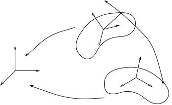
Figure A.1: Trajectory of a rigid body relative to a fixed frame.

Letting h = g−1 we see that, using left translation, the velocity of the rigid body can be shifted to the identity and written as a twist

Vb b = g−1g˙.

This is precisely the body velocity that was defined in Chapter 2.

If we use right translation to map a velocity g˙ Tg SE(3) to the tangent space at the identity, the resulting quantity is the spatial velocity:

Vb s = gg˙ −1.

The derivation of this formula follows exactly as in the body velocity case, replacing Lh with Rh.

One reason for the terminology “body” velocity and “spatial” velocity becomes clear if we consider the action of twists on points. Let q R3 be a point attached to a rigid body and let gab(t) SE(3) describe the trajectory of a frame B attached to the rigid body relative to a fixed reference frame A, as shown in Figure A.1. In homogeneous coordinates, the trajectory of the point q as a function of time can be written as

qa(t) = gab(t)qb,

where qa and qb are the coordinates of the point relative to the A and B frames. The velocity of the point, relative to the A frame, is given by

where we have used the fact that qb is constant since the point is fixed in the body frame. Thus, g˙ab(t) Tg SE(3) can be viewed as a mapping

419

between the body coordinates of a point and the spatial velocity of that same point.

A more appealing representation of velocity is one which does not require switching between coordinate frames. That is, suppose we wish to find the relationship between the coordinates of a point and its velocity, when both quantities are specified with respect to a single frame. We can accomplish this by transforming either the coordinates of the point or the coordinates of velocity to the appropriate frame. For example, if we are given the coordinates of the point q with respect to the spatial frame A, then the velocity of q with respect to A is given by

va = gq˙ b = (gg˙ −1)qa.

This is precisely the spatial velocity that is defined by using right translation to pull back the velocity g˙ Tg SE(3) to TeSE(3). A similar argument shows that the body velocity, g−1g˙ can be viewed as a map from the body coordinates of a point to the body velocity of that point.

The body and spatial velocities are physically interpreted as the instantaneous translational and rotational velocity written relative to the body or spatial frame, respectively. They are related to one another by

b b

the adjoint action of SE(3) on se(3). Namely, if V is the body velocity for a rigid motion g(t), then the spatial velocity is given by

This relationship can be derived by direct calculation, as in Chapter 2. A generalized force on SE(3) can be regarded as a covector on SE(3);

i.e., an element of Tg SE(3). As with velocities, we can map the cotangent space Tg SE(3) onto the dual of the Lie algebra by either left or right translation. We call the resulting object a wrench. Left translation corresponds to representing the force in the body coordinate frame while right translation corresponds to representing it in the spatial coordinate frame. The natural action of a wrench on a twist gives the instantaneous work due to applying the given wrench along the infinitesimal motion generated by the twist.

If we identify se(3) with R6, then a wrench can be written as

f

F = τ ,

where f is the translation component of the force and τ is the angular component. The natural action of a wrench on a twist becomes the inner product between F R6 and V R6. It is important to keep in mind, however, that this action is the natural action of a covector on a vector, and is defined independently of any inner product structure on

6 se(3).

R =

420

Although wrenches are dual to twists, we choose to represent them slightly di erently. We always represent a wrench on SE(3) as a vector in R6 since the matrix representation of a wrench does not prove to be particularly useful. Furthermore, we write a wrench using a single subscript to denote the frame with respect to which it is written. Thus, if A is an inertial reference frame and B is a frame attached to a rigid body, we write Fa for the spatial representation of a wrench applied to the rigid body and Fb for the body representation of the wrench. In taking the action of a wrench on a twist, one must always insure that the twist and the wrench are represented relative to the same frame. Thus the instantaneous work generated by a twist V and a wrench F can be written either as Vabs · Fa or Vabb · Fb.

Transformation laws

Let Vbcs R6 be the spatial velocity of a frame C relative to an inertial frame B and suppose that we wish to know the spatial velocity with respect to a di erent inertial frame, A. Using the definition of the spatial velocity, we have

and hence the velocity of the rigid body is transformed according to the adjoint action of SE(3) on se(3). If we represent the velocities as vectors in R6 then we write Vacs = Adgab Vbcs where Adg : R6 → R6 is the matrix

R pRb

Adg = 0 R .

Note that here we use the symbol Adg to represent the adjoint mapping both on se(3) R4×4 and on R6, which is isomorphic to se(3).

Suppose instead that we change the body coordinate frame. Let gab represent the configuration of the frame B relative to A and let gbc represent a fixed transformation corresponding to a new choice of body frame. The spatial velocity of C with respect to A is given by

Thus, changing the body coordinate frame does not a ect the spatial velocity of the object.

Similar relationships can be derived for body velocities. Changing the spatial coordinate frame does not a ect the body velocity of a rigid object. However, if gab represents the motion of the rigid body with respect to the frame A and gbc represents a new choice of body frame, then

421

Thus the adjoint action of SE(3) on se(3) represents the e ect of a change of body frame on the body velocity.

The transformations described above assume that new and old body or spatial coordinate frames have a fixed relative configuration. If we are given two rigid motions gab(t) and gbc(t), then in order to compute the velocity of frame C relative to frame A, we must add the velocities between the frames. This addition must occur in a single coordinate frame, and hence we use the adjoint mapping to transform the velocities appropriately. For example, the spatial velocity between frames A and C

is given by

Vacs = Vabs + Adgab Vbcs .

The adjoint mapping in the second term converts the instantaneous velocity Vbcs , which is written in the coordinates of frame B, into an instantaneous velocity written relative to frame A.

The coadjoint action is used to model the transformation of wrenches.

the coordinates of the wrench relative to a new fixed frame, B, are given

by

Fb = AdTg−1 Fa ab

where gab is the configuration of frame B relative to A. This expression follows directly from the definition of the coadjoint action given in the previous section.

3.2Metric properties of SE(3)

Since the Lie algebra of SE(3) can be identified with R6, there is an inner product structure on se(3) induced by the usual inner product on R6. However, it turns out that this inner product is not invariant under change of coordinate frame and hence can be misleading. Suppose, for example, that we are given two twists ξ1 R6 and ξ2 R6 that satisfy ξ1 · ξ2 = 0. If we transform the coordinate frame with respect to which the twists are written, then the twists transform as ξi′ = Adg ξi, where g SE(3) represents the change of frame. The inner product between the twists in the new coordinate frame is given by

If p 6= 0, then the dot product is not preserved and hence two twists which are orthogonal relative to one choice of coordinate frame may not be orthogonal relative to a di erent choice of frame.

This lack of frame independence has caused some confusion in the robotics literature, due to incorrect use of the inner product on R6 as an inner product in se(3). In this section we show that there is no inner

422