mls94-complete[1]

where the columns of K span the null space of Jh.

Equation (8.31) describes the grasp kinematics as a control system. The dynamic finger repositioning problem is to steer the system from an initial configuration (θ0, x0) to a desired final configuration (θf , xf ). The explicit location of the fingertip on the object at the initial and final configurations can be found by solving the forward kinematics of the system.

The general case of finding u1(t) and u2(t) such that the object and the fingers move from an initial to final position (while maintaining contact) can be very di cult. We point out two interesting special cases:

1.If the hand has no redundant degrees of freedom (i.e., K is not present) then it might be possible to move to an arbitrary loca-

tion/grasp using only u1. Moving just the contact location requires a carefully chosen closed loop path in x.

2.If we have redundant degrees of freedom, then we can move the fingers along the object while keeping the object position fixed (x˙ =

u1 = 0). In this case, we use only the vector fields in K to move the fingers.

In the second case, it is su cient to study the control of a single finger, since the fingers are decoupled if the object is held fixed. We concentrate here on the second case, which is considerably simpler.

4.2Steering using sinusoids

Consider the case of a single spherical finger rolling on a plane. The kinematics were derived in Chapter 7 and the associated control system is repeated here:

As in the preceding discussion, we will change variables to new ones and keep track of the Taylor series expansions of the nonlinear terms to get a two-chained system. More specifically, with change of state

z1 = q1 z2 = q2 z3 = −q5 z4 = q3 − q1 z5 = q4 + q2

383

0.0

-0.5

-1.0

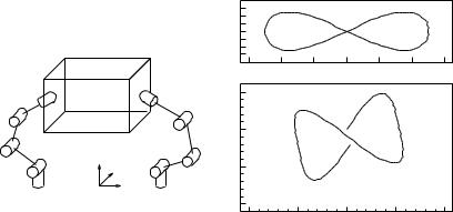
Figure 8.3: Steering applied to a multifingered hand.

where the ψi are quadratic or higher order in their respective arguments. If these functions ψi are neglected, then we have a two-chained system which can be steered using sinusoids. Unlike the case of the hopping robot or car parking, the calculation of the Fourier series coe cients for z4 and z5 is not easy. However, a numerical procedure based on using a sines and cosines at integrally related frequencies may be used to steer the finger on the surface of the object. An example of such a path moving a spherical fingertip down the side of a planar object is shown in Figure 8.3. In this figure, we consider the motion of a finger with a spherical tip on a rectangular object (left). The plots to the right of the figure show trajectories which move a finger down the side of the object. The location of the contact on the finger is unchanged as shown in the upper graph which plots the finger contact configurations (q1, q2) = (uf , vf ), while the location of the contact on the face of the object (q3, q4) = (uo, vo) undergoes a displacement in the vo direction.

384

4.3Geometric phase algorithm

In this subsection, we will describe the use of some techniques from classical di erential geometry which can be brought to bear on the specific problem of rolling a spherical finger on a planar surface.

As in Chapter 5, let Q be the configuration space of contact, Sf and S0 the surface of the fingertip and the object. Then, in local coordinates, Q is parameterized by η = (αf , αo, ψ), where αf = (uf , vf ), αo = (uo, vo) R2 are local coordinates on Sf and So respectively, and ψ is the angle of contact. The kinematic equations of rolling contact from Chapter 5 are

In the instance of a spherical finger rolling on a plane, we have that

where ρ is the radius of the finger. Since Mf and Rψ Mo are nonsingular, given either αf (t) R2 or αo(t) R2 there exists a unique path η(t) Q which satisfies the rolling without slipping constraint. More specifically, let αf (t), t [0, 1], be a path in Sf and denote u = α˙ f . Then the path η(t) Q is given by integrating the following di erential equations

This is to say that there exists a well defined lifting map ρ−1 : Sf → Q which lifts every path in Sf to a path in Q. The following classical theorem describes how a closed path in Sf generates a change in the angle of contact ψ. Using the formulas for Tf , Mf and To above yields

Note that this equation is independent of the radius ρ of the sphere. Thus, the following theorem, though stated for spheres of radius one, actually holds for spheres of arbitrary radius.

Theorem 8.6. Gauss-Bonnet theorem

Let αf : [0, 1] → Sf be a closed path on the sphere of radius one which encloses a cap shaped region Ω as shown in Figure 8.4. Let ψ be the change of the angle of contact as a result of rolling the sphere on the plane along the path given by αf (·). Then

385

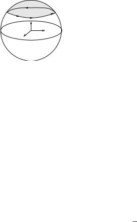
Ω

αf (t)

Figure 8.4: Geometric phase of a path in the sphere.

where the area of Ω is measured on the (curved) surface of the sphere of radius one.

Proof. From equation (8.36), we have that

˙ −

ψ = Tf Mf α˙ f = sin uf v˙f .

Z Z

= − cos uf dvf duf = − Area of Ω,

Ω

since cos uf duf dvf is the infinitesimal area (area form) on a sphere of radius one in local coordinates.

In the preceding theorem, we saw that the net change in the contact angle ψ depends on the area enclosed by the curve αf (·) on a sphere of radius one regardless of the actual radius of the sphere! ψ is referred to as the geometric phase or nonholonomy of the path αf (·). It tells us the motion (in fact the area to be covered by a closed path traced out by the finger) to generate a certain change in the contact angle ψ.

In the next proposition, we show how to generate motion on the spherical finger by using a closed path αo on the planar surface of the object. This specifies the motion of the object surface required to reposition the finger. In turn, we may use this method to produce closed loops in the motion of the finger, which produce changes in phase ψ. The development is completely geometric and does not use the rolling equation (8.35).

Proposition 8.7. Sphere rolling on a plane

Let αf and α˜f be two points on the sphere which are a distance l apart on the sphere. Assume that l < π2 . Then, rolling the sphere on the

386

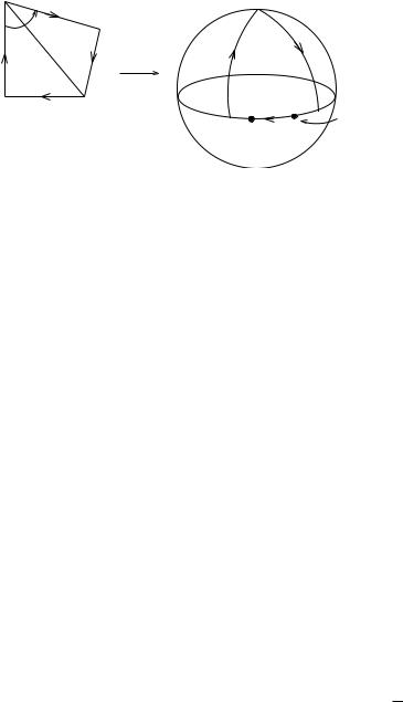
Figure 8.5: Closed path in the plane generates motion on the sphere.

plane along the closed curve ABCDA shown in Figure 8.5 takes αf to α˜f provided the segments AB, DA are of length x and BC, CD are of length π2 , and x solves the equation

Proof. Connect αf and α˜f by an arc of a great circle, and denote by A the starting point on the plane. Tracing the straight line from A to B and then to C on the plane induces a curve in the sphere which starts at αf , passes through B′, and then comes to the north pole, C′, as shown in the Figure 8.5. Since the distance traversed by the fingertip on the surface of the object is the same as the distance on the sphere, we have that the distance between αf and B′ is x and (αf B′C′) = π2 . Going from C to D at an angle θ and a distance π2 is equivalent to going down from C′ to some point D′ on the equator and d(B′, D′) = θ. By tracing a straight line from D to A on the plane, we follow the equator from D′ to some point α˜f , where d(α˜f , D′) = x. It is clear from the figure that

f (x) = l

has a unique solution x [0, π2 ] because f (0) = 0, f (π/2) = π/2 > l and f ′(x) > 0.

To summarize, using techniques from geometry and Green’s theorem one can generate strategies for rolling the planar surface of an object face to cause certain desired motion in the spherical fingertip and the angle of contact. The method appears to be ad hoc and specific to the

387

specific geometry of the finger and the object, however, it may in fact be generalized to other geometries. In fact, there is a generalization of the method to situations other than fingers rolling on objects called the method of geometric phase. For example, this method can be used to solve problems of reorienting satellites in space or to give an explanation for how cyclic motions of cilia on the surface of a paramecium cause forward motion in the paramecium.

388

5Summary

The following are the key concepts covered in this chapter:

1.Optimal controls (minimizing integral least squares cost) for steering a system with growth vector (2, 3) of the form

q˙1 = u1 q˙2 = u2

q˙3 = q1u2 − q2u1

are sinusoidal. Further more when q1(0) = q2(0) = q1(1) = q2(1) = 0, the optimal inputs are sinusoids at frequency 2π.

2. For a system of the form

q˙ = u

the optimal steering inputs, minimizing the integral least squares cost, are sinusoidal. Further, when q(0) = q(1) = 0 the optimal inputs are sinusoids at integrally related frequencies.

3.Using integrally related sinusoids as (sub-optimal) inputs, one can steer chained form systems. A one-chain system is one of the form

q˙1 = u1 q˙2 = u2 q˙3 = q2u1 q˙4 = q3u1

.

.

.

q˙n = qn−1u1

Generalizations to multi-chain systems also exist. Involutivity conditions for converting given control systems into the chained form may be given.

4.While it is di cult to give closed form expressions for the optimal controls associated with solving the least squares steering problem for a nonholonomic control system, one can derive formulas for the time derivatives of the optimal inputs. Further, numerical techniques, such as the Ritz approximation algorithm, may be used to derive approximate algorithms for generating the optimal controls.

5.Piecewise constant inputs can be used to steer a nonholonomic control system in the Philip Hall basis coordinates when the controllability Lie algebra is nilpotent.

389

6.Dynamic finger repositioning on the surface of an object can be carried out using sinusoids. In the special case of a spherical finger rolling on the surface of a flat object, the geometry of the GaussBonnet theorem may be used to position the finger on the object surface and adjust the angle of contact.

6Bibliography

While research in nonholonomic behavior of mechanical systems is quite classical, interest in steering and trajectory generation is quite recent. To our knowledge, the connection between nonholonomy and constructive controllability was first pointed by Laumond [55] in the context of mobile robots and Li [58, 60] in the context of fingers rolling on the surface of a grasped object. The literature in controllability for nonlinear systems is quite extensive. A good review of it is to be found in the textbooks of Nijmeijer and van der Schaft [83] and Isidori [43]. However, some of the most important first results on constructive controllability appeared in [11] and [4], where the least squares steering problem was solved for a class of model systems on Rn and SO(3) respectively.

In this chapter, we have used as source material some of our own recent publications in this area, such as [60] and [77] for steering fingers rolling on the surface of an object, [78] which discusses the use of sinusoids in steering nonholonomic systems, [103] which discusses the structure of optimal controls for steering problems, [32, 33] on the Ritz approximation procedure for solving optimal control problems, and [112] which solves the problem of parking a car with N trailers. A recent collection of papers [61] contains a good cross-section of papers on nonholonomic motion planning for further reading. A discussion of nonholonomic mechanics and geometric phase is in [67, 68].

390

7Exercises

1.Show that the following system

is controllable and nilpotent of degree four. Can you find a nonlinear change of coordinates to transform this system into a one-chained form?

2. Show that the following system is controllable and nilpotent:

q˙1 = u1 q˙2 = u2

q˙3 = q1u2 − q2u1

q˙4 = q12u2

q˙5 = q22u1.

3. Consider the following control system

q˙ = u

(a)Derive the Euler-Lagrange equations for the system, by minimizing the following integral

1 Z 1 uT u dt.

2 0

391

˜

(c) Find the input u to steer the system from (0, 0) to (0, Y )

Rm × so(m).

4. Consider the following system

q˙1 = u1 q˙2 = u2

q˙12 = q1u2

q˙121 = q12u1

q˙122 = q12u2

Apply the inputs

u1 = a1 sin 2πt + a2 cos 2πt + a3 sin 4πt + a4 cos 4πt u2 = b1 sin 2πt + b2 cos 2πt + b3 sin 4πt + b4 cos 4πt

to this system and integrate q˙121 and q˙122 from t = 0 to t = 1 to obtain a system of polynominal equations in (ai, bi). Propose a

method for solving for the coe cients (ai, bi) given the initial and final states.

5.Two-input two-chained system

The following system is referred to as a two-input, two-chained system

where y1 := x0y0 − x1 to account for skew-symmetry of the Lie bracket.

(d)Give an algorithm for steering the system from an initial state to a final state.

6.In the proof of Proposition 8.4, it was asserted that if u satisfies the di erential equation

u˙ = Ω(t)u

392