mls94-complete[1]

object held by the robot (e.g., the arc welder) as

Mo(x)¨x + Co(x, x˙ )x˙ + No(x, x˙ ) = 0,

where x Rp represents the workspace coordinates and the usual structural properties are satisfied by Mo and Co.

The kinematics of the mechanism is given by

˙

J (θ)θ = x,˙

which has the form of our canonical constraint with G = I Rp×p. Thus, we can write the dynamics as

F = J −T τ

(quantities with the subscript f refer to the robot dynamics). It follows

immediately that M > 0 and M − 2C is skew-symmetric.

The dynamics given in equation (6.26) represent the equations of mo-

the inertia of the system as viewed from the object frame of reference. As

˜

in the grasping case, M (q) incorporates both the object inertia and the inertia of the robot (at its current configuration). If the robot approaches a singular configuration, the inertia matrix becomes unbounded. This is because large workspace forces produce small object accelerations, and hence the e ective inertia appears very large. However, this singularity is strictly due to the parameterization of the dynamics in terms of the workspace coordinates. The dynamics of the mechanism in joint coordinates are never singular.

There are several variations on this problem. The dynamics can be written in terms of xo SE(3) by replacing x with xo, x˙ with Vob, and x¨

˙ b

with Vo (see the comments at the end of Section 2.1). We can also write the dynamics even if no object is present, by setting Mo, Co, and No to zero. This is useful if we simply wish to command the trajectory of a robot in end-e ector coordinates. Finally, we can in certain cases relax the assumption that J (θ) be square. This is discussed in more detail in Section 3.

The primary di erence between this class of examples and grasping is the lack of any “internal forces” (since G = I never has a null space).

283

Hybrid position/force dynamics

Another common manipulation task is one which consists of moving the robot in certain directions while pushing in other directions. An elementary example is writing on a chalkboard: the task specification consists of a desired motion in the plane of the chalkboard and a desired force against the chalkboard. A preliminary discussion of this topic is contained in Chapter 4. We now use the tools developed in this chapter to describe this situation more completely.

To analyze the kinematics of this system, we assume that the end- e ector is required to satisfy a holonomic constraint of the form

where x Rp parameterizes the allowable motions of the manipulator. For example, when writing on a chalkboard, x might specify the location of the chalk on the board as well as its orientation (in some suitable set of local coordinates). More generally, h(θ, x) specifies a p-dimensional surface in the configuration space of the manipulator. The task description consists of motion along this surface and generalized forces against this surface.

Equation (6.27) can be converted into the standard problem by differentiating with respect to time:

JGT

As before, we assume that J is square and nonsingular, indicating that no internal motions are present and that the manipulator is not at a singular configuration relative to the task. Internal forces correspond to joint torques τ such that GJ −T τ = 0. These are precisely the torques which generate forces against the constraint surface.

To formulate the dynamics of the mechanism, we assume that the object held by the robot is accounted for in the robot dynamics, and hence

F = GJ −T τ.

The reason for combining the object dynamics with those of the robot is that x Rp may not actually correspond to the configuration of an

284

object in many applications. For instance, in the chalkboard example, only two of the linear velocities are specified by x˙ . If the chalkboard were curved instead of flat, correctly specifying the object dynamics in terms of x becomes much more involved.

As with grasping, internal forces do not a ect the equations of motion and hence they can be ignored if only the free motion is to be studied. If internal forces are to be controlled or regulated, they can be found by solving for the Lagrange multipliers.

Several variations of this problem are possible. The use of local coordinates for motion which is constrained to a subgroup of SE(3) can be relaxed by appropriate interpretation of velocities and accelerations. In addition, the specifications of the task need not be in the form of a holonomic constraint. For some problems, it may be more natural to specify the kinematics directly in terms of J and G.

3Redundant and Nonmanipulable Robot Systems

In order to perform a given task, a robot must have enough degrees of freedom to accomplish that task. In the analysis presented so far, we assumed that our robots had exactly the number of degrees of freedom required to complete the task. That is to say, we assumed that each finger could follow the object through any allowable trajectory, but that the fingers had only the number of degrees of freedom required by the contact type (i.e., one degree of freedom for a frictionless point contact, three for a point contact with friction, and four for a soft-finger contact). This assumption manifested itself in our requirement that Jh be an invertible square matrix when we derived the dynamics. We now relax that requirement and discuss its consequences.

There are two situations in which Jh can fail to be square and invertible:

1.The manipulator has too many degrees of freedom. In this case,

Jh will have two or more columns which are linearly dependent, allowing internal motions which leave the contact locations fixed.

2.The manipulator has too few degrees of freedom. If Jh is not full row rank, it is not possible for the fingers to follow arbitrary motions of the contact points. This potentially limits the motion of the object, though it is possible for this situation to occur even if the grasp is manipulable.

These cases are not distinct; it is possible for a manipulator to have both internal motions and fail to be manipulable at the same time. In any case, we seek to cast the problem into the general framework developed in the

285

previous section by augmenting or decreasing the number of variables used to describe the task.

As before, we note that the material contained herein applies not only to multifingered hands, but to many other constrained systems as well. A few of these variations are described in the exercises.

3.1Dynamics of redundant manipulators

Unlike conventional robot manipulators, constrained robot manipulators do not need to have more than six degrees of freedom in order to be redundant. The constraints themselves can introduce kinematic redundancy into a system. For example, if we attach a six degree of freedom finger to an object using a soft-finger contact, we have introduced two redundant degrees of freedom: the finger is free to roll in either of two directions without a ecting the position of the object. Thus, it is absolutely essential that we include redundant mechanisms in our formulation.

It is interesting to note that there are actually two sources of redundancy introduced by our constraints: kinematic redundancy and actuator redundancy. Kinematic redundancy refers to motions of the fingers which do not a ect the motion of the object. Actuator redundancy refers to forces applied by the fingers which do not a ect the object motion, i.e., internal forces. The grasping constraint

contains all the information necessary to determine these redundancies. Namely, the null space of Jh describes the set of joint motions which do not a ect the motion of the object and the null space of G is precisely the space of internal forces. Since we have already discussed internal forces, we restrict our discussion to kinematic redundancy.

Consider first the kinematics of a single redundant manipulator, with no constraints. If we are willing to control the manipulator in joint space, the dynamics formulation presented above holds without modification. However, in order to perform a task specified in terms of the configuration of the end-e ector, we must first choose a joint trajectory which accomplishes this task. Suppose instead that we wish to write our controllers directly in end-e ector coordinates. We represent the kinematics as a function g : Rn → SE(3). In this case, the manipulator Jacobian

cannot write θ in terms of Vst as we did previously.

It is still possible to write the dynamics of redundant manipulators in a form consistent with that derived earlier. To do so, we define a matrix K(θ) R(n−p)×n whose rows span the null space of J (θ). As before, we assume that J (θ) is full row rank and hence K(θ) has constant rank n − p. The rows of K(θ) are basis elements for the space of velocities

286

which cause no motion of the end-e ector; we can thus define an internal motion, vN Rn−p, using the equation

If we choose K such that its rows are orthonormal and also perpendicular

Note that we have parameterized the internal motion of the system by a velocity and not a new variable y. We do this out of necessity: since we chose K only to span the null space of J , there may not exist a function

is merely the statement that mixed partials of h must commute. A more thorough treatment of this point is given in Chapter 7, and is illustrated briefly in the next example.

In general, it may not always be easy to choose K(θ) such that it is the di erential of some function. For this reason, we shall not generally assume that an explicit coordinatization of the internal motion manifold is available. Thus, in the same way as we were forced to use velocity relationships when modeling constraints, we also use velocity relationships for redundant manipulators. The Lagrange-d’Alembert formalism lets us treat this case without di culty.

Example 6.3. Three-link planar manipulator

Consider a three-link planar manipulator with unit-length links, as shown in Figure 6.5. If we let (x, y) be the location of the end-e ector, then

x = cos θ1 + cos θ2 + cos θ3 y = sin θ1 + sin θ2 + sin θ3,

287

θ3

θ1

B

Figure 6.5: Three-link planar manipulator with joint angles measured relative to the horizontal axis.

where the link angles are all with respect to a fixed (inertial) axis. The Jacobian of the mapping θ 7→(x, y) is

the end-e ector to parametrize internal motions. This choice of K(θ) is valid as long as θ1 6= θ2 (i.e., when the first two links are not aligned). If, on the other hand, we choose

Hence, there is no h such that not the derivative of a variable y.

We now derive the equations of motion for the system in terms of x, y, and vN . Let M (θ) be the inertia matrix for the manipulator in joint

˙

space with C(θ, θ), the corresponding Coriolis matrix. For brevity, we ignore the potential and nonconservative forces. The dynamics of the

288

where

We now return to the general case and extend our treatment to include the full grasp constraints. Consider a force-closure and manipulable grasp with velocity constraints

where N(Jh) 6= ′. As before, we augment the constraint by choosing a matrix Kh(θ) whose rows span the null space of Jh(θ). The grasp constraint can now be written as

where Jh and G represent the augmented hand Jacobian and grasp matrix. This constraint has the same form as the standard (nonredundant)

We now see that redundant manipulators can be incorporated into the same general framework as other robot systems. The necessity of augmenting the description of the system stems from our use of the task variables, parameterized by x, to specify the motion of the system. Since the mechanism is redundant, the x variables alone do not provide su - cient information to determine the motion of the system. Augmenting the task description with the variables vN gives a complete description of the motion of the system.

One final comment is in order regarding the relationship between the joint torques and the object wrench for a redundant grasp. In Chapter 5, we derived the static relationships between the joint torques, the contact forces, and the object wrench. These relationships were used to determine how to push on an object, via the fingers, in order to resist applied forces.

289

In the redundant case, a bit of care must be taken in interpreting these results.

Consider the general grasping situation described above. Reverting to twists, the kinematic constraints have the form

The forces fN parameterize the forces which correspond to internal motions vN . If these forces are chosen to be zero, then we retrieve the usual force relationships between joint torques and object wrenches.

If the forces fN are not chosen to be zero, then the manipulator will begin to exhibit internal motions. This motion can cause accelerations of the manipulator joints and we can no longer use equation (6.31) to represent the force relationships in the system. Instead, we must consider the full equations of motion as given in equation (6.30). In particular, the internal motions of the system may generate constraint forces and hence the relationships in equation (6.31) are no longer correct. This situation does not occur in nonredundant systems since if we keep the end-e ector fixed, then all joint angles also remain fixed and hence no dynamic terms are present.

3.2Nonmanipulable grasps

We now consider the situation in which the hand Jacobian is not full row rank. In this case, there are some motions of the individual contacts which cannot be tracked by the fingers. We assume that the hand Jacobian is full column rank. If not, the methods of the preceding subsection can be used to augment the grasp with appropriate internal velocities.

In most situations, if the hand Jacobian is not full row rank, then the grasp fails to be manipulable. However, in certain special situations, it is possible that a multifingered grasp is both manipulable and nonredundant but Jh is not square. This can occur when the structure of the grasp is such that Jh is bijective onto the range of GT but is not surjective as a map from Rn → Rm. This situation almost never occurs in practice, and hence we concentrate here only on the case where Jh is nonmanipulable.

To treat the nonmanipulable case, we must restrict the motions of the object to those which can be accommodated by the fingers. This restriction is enforced by structural forces within the hand, which resist motion of the system in directions in which the fingers are unable to move.

290

As usual, our formulation assumes that the contacts are maintained and hence the contact forces must remain inside the friction cone at all times. It is the responsibility of the control law to insure that this condition holds at all times.

Consider a nonmanipulable grasp with grasp constraint

Let W (θ, x) represent the space of allowable object velocities,

We assume that W (θ, x) has constant dimension l > 0 and that W varies smoothly as a function of its arguments. Choosing a matrix H(θ, x) Rp×l whose columns span W (θ, x), we can write the grasp constraints as

x˙ = Hw,

where w Rl represents the object velocity in terms of the basis formed by the columns of H.

and Jh+T is the transpose of Jh+. The second-order dynamics in equation (6.33) combined with the first-order constraints in equation (6.32) give a complete description of the motion of the system.

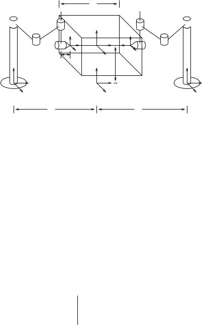
3.3Example: Two-fingered SCARA grasp

To illustrate the results of this section, we consider the dynamics of two SCARA fingers grasping a box, as shown in Figure 6.6. Each finger is

291

Figure 6.6: Two-fingered grasp using SCARA robots.

modeled as a soft-finger finger contact. The fundamental grasp constraint for the system has the general form

←−−−−−−→ ←−−→

88

Although Jh(θ) R8×8 is a square matrix, it is not invertible. It was shown in Section 5.3 of Chapter 5 that the grasp is not manipulable and also contains internal motions. The lack of manipulability comes from the fact that rotations about the line connecting the contacts violate the softfinger contact constraints. The internal motions correspond to motions of the first three joints of each finger which leave the xy positions of the fingertips fixed.

To parameterize the internal motion of the system, we augment the system using the angles of the last joint of the fingers, as in Example 6.3.

Letting y = (θ11 + θ12 + θ13, θ21 + θ22 + θ23), the contact constraints become

Note that for this example we were able to choose actual variables to parameterize the internal motions and not just velocities.

292