∂c
∂u
 v
v
 O
O
R2
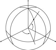
Figure 5.18: Surface chart for a two-dimensional object in R3.
formulation to moving contacts. The formulation here covers rolling between smooth fingers and smooth objects. It does not cover scenarios in which fingers roll on the edge of an object, but extensions to this case are possible. We begin with a brief description of surface parameterizations.
6.1Surface models
Given an object in R3, we describe the surface of the object using a local coordinate chart, c : U R2 → R3, as shown in Figure 5.18. The map c takes a point (u, v) R2 to a point x R3 on the surface of the object, written in the object frame of reference, O. Thus, locally, we can describe a point on the surface by specifying the corresponding (u, v). In general, it may take several coordinate charts to completely describe the surface of the object. A surface S is regular if for each point p S there exists a neighborhood V R3, an open set U R2, and a map c : U → V ∩ S such that
1.c is di erentiable.
2.c is a homeomorphism from U to V ∩ S. That is, c is continuous, bijective (one-to-one and onto), and has a continuous inverse.
3.For every α = (u, v) U , the map ∂α∂c (α) : R2 → R3 is injective (one-to-one).
At any point on the object, we can define a tangent plane which consists of the space of all vectors which are tangent to the surface of the object at that point. The tangent plane is spanned by the vectors cu := ∂u∂c and cv := ∂v∂c . That is, any vector which is tangent to the
243
surface at a point c(u, v) may be expressed as a linear combination of the vectors cu and cv , evaluated at (u, v). A coordinate chart is an orthogonal coordinate chart if cu and cv are orthogonal.
Theorem 5.9. Locally, there exists an orthogonal chart for all regular surfaces.
The proof can be found in any standard book on di erential geometry.
In the sequel, we will make frequent use of some more detailed concepts from di erential geometry. Although the application of the rolling equations does not require knowledge of these concepts, they do allow a deeper understanding of the material. We present here a brief review of the relevant topics; a full description can be found in DoCarmo [27].
In order to define the area of a surface, one needs to define the inner product between two tangent vectors on the surface. This defines the area of a parallelogram and the total area can then be calculated by integrating the infinitesimal areas generated by parallelogram-shaped patches on the surface. The first fundamental form for a surface describes how the inner product of two tangent vectors is related to the natural inner product on R3. In a local coordinate chart, it is represented by a quadratic form Ip : R2 × R2 → R which takes two tangent vectors attached at a point p = c(u, v) and gives their inner product. If c is a local parameterization, then the matrix representation of the quadratic form is given by
cuT cu |
cuT cv |
. |
|
Ip = cvT cu |
cvT cv |
(5.17) |
We will use the symbol Ip to represent both the quadratic form and its matrix representation. Note that each element of Ip is an inner product between vectors in R3 and that Ip is symmetric and positive definite. If a parameterization is orthogonal, only the diagonal terms are nonzero.
The first fundamental form can be used to define the metric tensor for a surface. The metric tensor is given by the square root of the first fundamental form and is used to normalize tangent vectors. We define the matrix Mp : R2 → R2 as the positive definite matrix which satisfies
Ip = Mp · Mp.
In the case that the parametrization is orthogonal, Mp has the form
Mp = |
kcuk |
0 |
. |
(5.18) |
|
0 |
kcv k |
|
|
(The metric tensor described here is the square root of the Riemannian metric used in di erential geometry.)
At each point on a surface S, we can define an outward pointing unit normal by taking the cross product between the vectors that define the

tangent space. We identify the set of all unit vectors in R3 with S2, the unit sphere in R3. The Gauss map N : S → S2 gives the unit normal at each point on the surface S. In local coordinates,
|
N (u, v) = |
cu × cv |
|
. |
(5.19) |
|
|cu × cv |
| |
|
|
|
|
For smooth, orientable surfaces, the Gauss map is a well defined, di erentiable mapping. We write n = N (u, v) for the unit normal at a point on the surface.
The directional derivative of the Gauss map defines the second fundamental form for a surface. The second fundamental form is a measure of the curvature of a surface. In a local coordinate chart, it is represented by a map IIp : R2 × R2 → R: which has a matrix representation
cT n |
u |
cT n |
v |
, |
|
u |
u |
|
IIp = cvT nu |
cvT nv |
(5.20) |
where p = c(u, v), nu := ∂n∂u , and nv := ∂n∂v . This matrix describes the rate of change of the normal vector projected onto the tangent plane. It
may be interpreted as follows: if p(s) S is a curve lying on S that is parameterized by arc length and whose tangent vector is p′, then (p′)T IIpp′ gives the usual curvature of the spatial curve p.
For our purposes, it will be convenient to scale the second fundamental form and define the curvature tensor for a surface. For an orthogonal set of coordinates, the curvature tensor is a mapping K : R2 → R2 defined
as |
= |
cT n |
|
|
|
|
|
cT n |
|
. |
|
|
u |
|
|
|
|
|
|
|
u |
|
|
|
u |
v |
|
|
Kp = Mp−T IIpMp−1 |
c |
2 |
|
k |
cu |
cv |
k |
|
|
|
|
kTu k |
|
|
|
Tkk |
|
|
(5.21) |
|
|
|
cv nu |
|
|
|
cv nv |
|
|
|
|
kcu kkcv k |
|
|
|
kcv k2 |
|
|
|
|
|
|
|
|
|
|
|
|
|
|
|
|
|
The factors of Mp−1 are normalization factors which account for scaling present in the local coordinate chart for the surface.
The curvature tensor can also be computed in terms of a special coordinate frame called the normalized Gauss frame. If c(u, v) is an orthogonal chart, then we define the normalized Gauss frame as
|
|
|
= h |
cu |
|
cv |
|
ni . |
|
x y |
z |
|
kcu k |
|
kcv k |
(5.22) |
The normalized Gauss frame provides an orthonormal frame at each point on the surface. In terms of this frame, the curvature tensor is given by
xT |
h |
nu |
|
nv |
|
Kp = yT |
|
|
|
i , |
(5.23) |
kcu k |
kcv k |
which can be interpreted as a measure of how the unit normal varies across the surface, as projected on the tangent plane. Again, a normalization

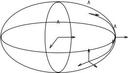
Figure 5.19: The contact frame is a moving frame along a curve p(t).
factor is present to account for scaling due to the parameterization. If the surface is flat, then nu = nv = 0 and Kp = 0.
Finally, we define the torsion form. For a curve, the torsion measures the rate of change of curvature along the curve. The torsion of a surface is a measure of how the Gauss frame twists as we move across the surface, again projected onto the tangent plane. To compute the torsion, we only need to keep track of how either x or y changes, since they are orthonormal. We define the torsion form T : R2 → R as
|
T |
|
xu |
|
xv |
|
|
cT cuu |
|
cvT cuv |
|
|
|
|
|
|
Tp = y |
|
h kcu k |
kcv k i |
= h |
v |
|
|
i , |
(5.24) |
|
kcu k2kcv k |
kcu kkcv k2 |
where xu and xv denote the partial derivative of x with respect to u and v,
cuu := ∂u∂2c2 , and cuv := ∂u∂v∂2c . Note that the torsion form is represented as a row vector, not a matrix. The torsion form is related to the Christo el
symbols for a surface parameterization (see [27]). If a surface is flat, then Tp = 0.
Given a parameterization, (Mp, Kp, Tp) are collectively referred to as the geometric parameters of the surface. These parameters describe the local geometry of the surface and play an important role in the kinematics of contact which we will pursue in the section that follows.
Let p(t) S be a curve on the surface of the object and define the contact frame along the curve to be the frame C which coincides with the Gauss frame at time t (see Figure 5.19).2 We wish to determine the motion of the contact frame as a function of the geometric parameters and the velocity of the curve. If we fix a frame O in the object then the motion of the frame C is given by the rigid transformation goc(t) SE(3). We assume p(t) lies in a single coordinate chart c : U → R3 and we let α(t) = c−1(p(t)) represent the local coordinates.
Lemma 5.10. Induced velocity of the contact frame
The (body) velocity of the contact frame C relative to the reference frame
2This is di erent from our previous convention, where we choose the z-axis along the inward pointing normal.
Oof the object is given by Vocb = (voc, ωoc) where
|
|
|
|
|
voc = |
M α˙ |
|
|
|
|
(5.25) |
|
|
|
|
|
|
|
|
0 |
|
|
|
|
|
ωoc = |
ωz |
−0 z |
−ωx |
= |
T M α˙ |
− |
0 |
KM α˙ |
, |
|
|
|
0 |
ω |
ωy |
|
|
|
0 |
|
T M α˙ |
|
|
|
|
|
|
|
|
|
|
|
|
|
|
b |
|
|
|
|
|
|
|
|
|
|
|
|
|
|
|
|
|
|
|
|
−ωy |
ωx |
0 |
−(KM α˙ )T |
0 |
|
|
|
(5.26) |
|
|
|
and M , K, and T are the geometric parameters of the surface relative to the coordinate chart (c, U ).
Proof. The position and orientation of the contact frame relative to the reference frame are given by
poc = p(t) = c(α(t)) |
|
|
|
|
××cv k i . |
Roc = |
x(t) y(t) z(t) = h kcu k kcv k kcu |
|
|
cu |
|
cv |
|
cu |
cv |
The translational component of the body velocity is given by voc = RocT p˙oc which yields
voc = |
yT |
∂α α˙ = |
yT cu |
|
xT |
∂c |
xT cu |
|
zT |
zT cu |
|
|
|
To show equation (5.26), we compute the body angular velocity:
ωoc = RocT R˙ oc = |
yT |
x˙ |
y˙ z˙ = |
yT x˙ |
0 |
yT z˙ |
|
, |
b |
xT |
|
|
0 |
xT y˙ |
xT z˙ |
|
zT |
|
zT x˙ |
zT y˙ |
0 |
|
|
where the zero entries follow because x, y, and z are unit vectors. Now using the definitions of K, T , and M we have
ωoc = |
T M α˙ |
− |
0 |
KM α˙ |
. |
|
|
0 |
|
T M α˙ |
|
|
b |
|
|
|
|
|
−(KM α˙ )T |
0 |
Example 5.6. Geometric parameters of a sphere in R3
A coordinate chart for the sphere of radius ρ can be obtained by using spherical coordinates, as shown in Figure 5.20. For the hemisphere centered about the x-axis, we have
ρ cos u cos v c(u, v) = ρ cos u sin v ,
ρ sin u
z
u
v
Figure 5.20: Spherical coordinate chart for a sphere.
with
U = {(u, v) : −π/2 < u < π/2, −π < v < π}.
The partial derivatives of c with respect to u and v are given by
cu = |
−ρ sin u sin v |
|
|
ρ sin u cos v |
|
− ρ cos u |
|
−ρ cos u sin v cv = ρ cos u cos v
0
and we see that cTu cv = 0 and hence the chart is orthogonal. The curvature, torsion, and metric tensors are:
K = 10 |
1/ρ |
M = 0 |
ρ cos u |
T = |
0 |
−1/ρ tan u . |
/ρ |
0 |
ρ |
0 |
|
|
|
|
|
|
6.2Contact kinematics
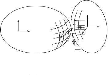
Consider two objects with surfaces So and Sf which are touching at a point, as shown in Figure 5.21. We are interested in the motion of the points of contact across the surfaces of the objects in response to a relative motion of the objects.
Let po(t) So and pf (t) Sf be the positions at time t of the point of contact relative to two body-fixed frames O and F , respectively. For simplicity, we will restrict ourselves to the case where motion is contained in a single coordinate chart for each object. Let (co, Uo) and (cf , Uf ) be
charts for the two surfaces, and αo = c−o 1(po) Uo and αf = c−f 1(pf ) Uf be local coordinates. We will assume that co and cf are orthogonal
representations of the surfaces. Let ψ be the angle of contact, defined as
|
the angle between the tangent vectors |
∂cf |
and |
∂co |
. We choose the sign of |
|
∂uf |
∂uo |
|
|
|
|
|
|
ψ so that a rotation of |
∂co through an angle ψ around the outward normal |
|
|
∂uo |
|
|
|
|
no
 O
O
F
∂co  ∂uo ψ
∂uo ψ
∂cf
∂uf
Figure 5.21: Motion of two objects in contact.
of So aligns ∂co with ∂cf (see Figure 5.21). Collecting the quantities
∂uo ∂uf
which describe the contact, we call η = (αf , αo, ψ) the contact coordinates for Sf and So.
Let gof SE(3) describe the relative position and orientation of Sf with respect to So. We wish to study the relationship between gof and the local contact coordinates. To do so, we assume that gof W SE(3), where W is the set of all relative positions and orientations for which the two objects are in contact.
The coordinate charts (co, Uo) and (cf , Uf ) induce a normalized Gauss frame at all points in co(Uo) So and cf (Uf ) Sf . We define the contact frames Co and Cf as the coordinate frames that coincide with the normalized Gauss frame at po(t) and pf (t), for all t I, where I is the interval of interest. We also define a continuous family of coordinate frames, two for each τ I, as follows. Let the local frames Lo(τ ) and Lf (τ ), be the coordinate frames fixed relative to O and F , respectively, that coincide at time t = τ with the normalized Gauss frame at po(t) and pf (t) (see Figure 5.22).
We describe the motion of O and F at time t using local coordinate frames Lo(t) and Lf (t). Let vlo lf = (vx, vy , vz ) be the components of the (body) translational velocity of Lf (t) relative to Lo(t) at time t. Similarly, let ωlo lf = (ωx, ωy , ωz ) be the (body) rotational velocity. Here (ωx, ωy ) are the rolling velocities along the tangent plane at the point of contact, and ωz is the rotational velocity about the contact normal. Likewise, (vx, vy ) are the linear velocities along the tangent plane, i.e., the sliding velocities, and vz is the linear velocity in the direction contact normal. As long as the two bodies remain in contact, vz = 0. In addition, for pure rolling contact we have vx = vy = 0 and ωz = 0 and for pure sliding contact we have ωx = ωy = ωz = 0. Since the local frames are fixed relative to their respective frame of reference, according

 Lo(τ1)
O 
 Lo(t) = Co
Lo(τ2)
Figure 5.22: Relation between the one-parameter family of local frames, Lf (t), and the contact frame, Cf . At time t I, Lf (t) coincides with
Cf .
to Proposition 2.15 we have Vlo lf
|
|
|
vy |
|
|
|
|
|
|
vx |
|
|
Vlo lf |
= |
|
|
= |
ω |
x |
|
|
|
|
|
|
|
b |
|
|
|
ω |
|
|
|
|
|
|
vz |
|
|
|
|
|
|
y |
|
|
|
|
|
ω |
z |
|
|
|
|
|
|
|
|
|
We also let |
|
|
|
|
|
|
|
− sin ψ |
− cos ψ |
Rψ = |
cos ψ |
− sin ψ |
= Adg−1 Vof or, in components, |
|
|
f lf |
|
|
" |
RfTlf ωof b |
# |
|
|
RfTlf vof − RfTlf poωof |
. |
(5.27) |
˜
and Ko = Rψ KoRψ .
Note that Rψ is the orientation of the x- and y-axes of Cf relative to
˜
the x- and y-axes of Co. Thus, Ko is the curvature of O at the point of
˜
contact relative to the x- and y-axes of Cf . We call Kf + Ko the relative curvature form.
Theorem 5.11. Kinematic equations of contact [72]
The motion of the contact coordinates, η˙, as a function of the relative motion is given by
f |
|
|
ωx |
|
− |
|
vy |
|
|
|
α˙ f = M −1(Kf + K˜o)−1 |
−ωy |
|
|
K˜o |
vx |
|
|
o |
|
|
ωx |
|
vy |
(5.28) |
α˙ o = M −1Rψ (Kf + K˜o)−1 |
−ωy + Kf |
vx |
|
˙ |
+ ToMoα˙ o |
|
|
|
|
|
|
|
ψ = ωz + Tf Mf α˙ f |
|
|
|
|
|
|
|
0 = vz , |
|
|
|
|
|
|
|
|
|
|
where (vx, vy , vz , ωx, ωy , ωz ) = V b |
= Ad−1 |
|
V b . |
|
|
|
|
|
lo lf |
|
gf lf |
of |
|
|
|
|
Before presenting the proof of the theorem, let us note that the equations of contact only make sense when the relative curvature is nonsingular. An example of a singular relative curvature occurs when one object is concave and the other is convex, and both have the same radius of curvature. In this case, small motions of the object can cause large motions of the contact and continuity is lost. To avoid this possibility, we shall assume that all manipulation occurs in an open set on which the relative curvature is invertible.
Proof of theorem. We perform all calculations using body velocities and hence temporarily drop the superscript b. Since the frame Lf (t) is fixed relative to the frame F , the velocity of Lf (t) relative to F is given by Vf lf = 0. Therefore, using the velocity relationships from Chapter 2,
Vf cf |
= Adg−l1c |
f |
Vf lf |
+ Vlf cf |
= Vlf cf . |
(5.29) |
|
|
f |
|
|
|
|
|
|
|
|
Similarly, we find that |
|
|
|
|
|
|
|
|
|
|
V |
oco |
= Ad−1 |
|
V |
olo |
+ V |
lo co |
= V |
lo co |
. |
(5.30) |
|
glo co |
|
|
|
|
|
We now compute the velocity of Cf relative to Lo(t) via two intermediate frames, namely Lf (t) and Co.
At time t, the position and orientation of Cf relative to Lf (t) are plf cf = 0 and Rlf cf = I. Thus,
Vlo cf = Vlo lf + Vlf cf
and since pco cf = 0,
Vlo cf = |
0 RcTo cf Vlo co + Vco cf . |
|
RT |
0 |
|
co cf |
|
Combining equations (5.29) through (5.32) yields
Vlo lf + Vf cf = |
0 RcTo cf Voco + Vco cf . |
|
RT |
0 |
|
co cf |
|
We now find the values of each of the quantities in equation (5.33) in terms of the geometric parameters and motion parameters. First, we observe that
pco cf |
= 0 |
1 |
|
vco cf |
= 0 |
i |
|
Rco cf |
= |
0 |
ωco cf |
= h ψ˙ |
|
|
|
Rψ |
0 |
= |
|
0 |
|
(5.34) |
|
|
|
|
|
|
0 |
|
|
and, by definition, Vlo lf = (vx, vy , vz , ωx, ωy , ωz ).
Second, according to Lemma 5.10,
|
|
|
|
|
|
|
|
|
|
|
|
|
|
vf cf |
= |
Mf α˙ f |
|
|
|
|
|
|
|
|
|
|
|
|
|
0 |
|
|
|
|
|
|
|
|
|
ωf cf |
= |
Tf Mf α˙ f |
− f 0 f |
α˙ |
f |
Kf Mf α˙ f |
|
(5.35) |
|
|
|
|
|
0 |
T M |
|
|
|
|
|
b |
|
|
|
|
|
|
|
|
|
|
|
|
|
|
|
−(Kf Mf α˙ f )T |
|
|
|
0 |
|
|
and |
= |
|
|
0 |
|
|
|
|
|
|
|
|
|
voco |
|
|
|
|
|
|
|
|
|
|
|
Moα˙ o |
|
|
|
|
|
|
|
|
|
|
|
|
|
0 |
M α˙ |
|
|
|
. |
|
|
|
|
|
|
|
|
ωoco |
= |
ToMoα˙ o |
−To 0 o o |
|
KoMoα˙ o |
(5.36) |
b |
|
|
|
−(KoMoα˙ o)T |
|
|
|
0 |
|
|
Substituting equations (5.34) through (5.36) into equation (5.33) and equating components, we get
|
0 |
|
+ |
vy = |
|
|
0 |
|
|
|
|
|
|
vz |
|
|
|
|
|
|
|
|
|
Mf α˙ f |
|
vx |
|
|
Rψ Moα˙ o |
|
Kf Mf α˙ f |
|
|
|
|
. |
|
+ |
−ωx |
= |
0 |
|
|
|
Rψ KoMoα˙ o |
|
|
|
|
|
|
|
|
|
|
0 |
|
|
|
|
|
(5.37) |
|
|
|
|
|
ωy |
|
|
|
|
|
|
|
|
|
|
Tf Mf α˙ f |
|
|
|
|
|
|
ψ˙ |
|
|
− |
|
ToMoα˙ o |
|
|
|
|
|
ωz |
|
|
|
|
|
|
|
|
|
|
|
|
|
|
|
|
|
|
|
|
After some algebraic manipulation, we can write equation (5.37) in the form given by equation (5.28). 

A common situation in grasping is to assume that the fingers roll without slipping on the object. In this case we can simplify the contact kinematics.
Corollary 5.11.1. The contact coordinates for rolling contact
according to |
ωx |
|
|
f |
|
α˙ f = M −1(Kf + K˜o)−1 |
−ωy |
|
|
o |
ωx |
α˙ o = M −1Rψ (Kf + K˜o)−1 −ωy |
|
˙
ψ = Tf Mf α˙ f + ToMoα˙ o.
Example 5.7. Sphere rolling on a plane
Consider a spherical finger of radius ρ rolling on a plane, as shown in Figure 5.23. The local coordinates of the plane are chosen to be co(u, v) =