mls94-complete[1]

We can further simplify the equations by reusing the constraints to eliminate x˙ , y˙ and x¨, y¨. Di erentiating the constraints, we have

and substituting into equation (6.12) gives

which describes the motion of the system as a second-order di erential equation in θ and φ. Note that for this system the equations of motion for θ and φ do not depend on x and y, but in general this is not the case.

The motion of the x and y positions of the disk can be retrieved from the first-order di erential equations

˙

x˙ = ρ cos θφ

˙

y˙ = ρ sin θφ.

Thus, given the trajectory of θ and φ, we can determine the trajectory of the disk as it rolls along the plane. The splitting of the equations of motion into a set of second-order equations in a reduced set of variables plus a set of first-order equations representing the constraints is characteristic of nonholonomic systems.

1.4The nature of nonholonomic constraints

The machinery that we have developed in this section allows us to calculate the dynamics of a mechanical system subject to a set of Pfa an constraints without trying to integrate the constraints and find a set of generalized coordinates which completely (and minimally) parameterize the configuration of the system. In the case that the constraints are integrable, these equations are identical to those obtained by finding a set of appropriate generalized coordinates. When the constraints are nonintegrable, it is very important to incorporate the constraints in the proper

274

way. In this section, we try to shed some light on how nonintegrable constraints a ect the mechanics of the system and indicate what can go wrong if one is not careful.

A common mistake when deriving the equations of motion for a mechanical system with nonholonomic constraints is to substitute the constraints into the Lagrangian and then apply Lagrange’s equations. This would seem to eliminate the dependent variables and minimize computations. As we shall see in a moment, however, this gives the wrong equations of motion for the system. We have been very careful in this section to always compute the unconstrained Lagrangian, substitute into the Lagrange-d’Alembert equations, and then reapply the constraints to eliminate the dependent variables.

To see what happens when the constraints are used at the wrong time, consider a three-dimensional, unforced Pfa an system with configuration q = (r, s) R2 × R, constraint

s˙ + aT (r)r˙ = 0 a(r) R2,

and Lagrangian L(r, r,˙ s˙). For simplicity, we assume that both the Lagrangian and the constraints do not depend on the variable s. Define the constrained Lagrangian as

Lc(r, r˙) = L(r, r,˙ −aT (r)r˙).

The constrained Lagrangian is the kinetic minus potential energy of the system, but evaluated with the constraints taken into account.

Suppose we substitute the constrained Lagrangian into the Lagrange- d’Alembert equations. Since there is no dependence on either s or s˙, these equations yield

Expanding the equations using the definition of Lc, we obtain

(6.15) Notice that the left-hand side of this equation is exactly the Lagrange-

d’Alembert equation for the system. The right-hand side of the equation represents spurious terms that arise from substituting the constraints

275

into the Lagrangian. This shows that, in general, substituting a set of Pfa an constraints into the Lagrangian and then applying the Lagrange- d’Alembert equations gives the wrong equations.

Suppose now that the constraint is actually holonomic. For simplicity, we assume that the constraint is explicitly integrable, so that there exists a function h(r) such that

which is identically zero since mixed partials commute. Hence, if the constraints happen to be holonomic, then substituting the constraints into the Lagrangian will give the correct equations of motion.

2Robot Hand Dynamics

Using the results from the previous section, we now derive the equations of motion for a system of robots performing a coordinated task. We begin with a multifingered hand manipulating an object and then show how the same formalism can be applied to other problems.

2.1Derivation and properties

The overall dynamics for a multifingered hand grasping an object are obtained by combining the dynamics of the fingers and the object via the grasp constraint. Adopting the notation of the previous chapters, the finger dynamics have the form

Mf , Cf , and Nf are formed by appropriately stacking the quantities

The object dynamics are given by the Newton-Euler equations, derived in Chapter 4. These equations have the form

276

where V b = (vb, ωb) is the body velocity of the object, F b is the body wrench, m is the mass, and I is the moment of inertia matrix, all with respect to a frame attached at the center of mass. We write xo = (p, R) for the configuration of the object. If the object is subject to gravity alone, the dynamics can be written as

where ~g is a vector in the direction of gravity, usually taken to be ~g = (0, 0, 1).

In order to apply the Lagrange-d’Alembert equations, it is necessary to rewrite the Newton-Euler equations in local coordinates. Letting x R6 be a local parameterization for xo SE(3), the object dynamics can be written as

Mo(x)¨x + Co(x, x˙ )x˙ + No(x, x˙ ) = 0,

which has the same form as the robot dynamics in equation (6.16). It

written here in local coordinates. We make three assumptions about the structure of the grasp:

1.The grasp is force-closure and manipulable. Recall that this is equivalent to the conditions

G(F C) = Rp and R(GT ) R(Jh)

for all possible configurations.

2.The hand Jacobian is invertible. This condition insures that there are no redundant motions of the fingers and hence the hand has exactly the number of degrees of freedom required to complete the task.

3.The contact forces remain in the friction cone at all times. This condition is necessary in order to insure that the grasp constraints in equation (6.18) hold at all times. It is the task of the control law to insure that this condition holds, since otherwise the object can slip or drop from the grasp.

The first two assumptions can be relaxed; we discuss those cases in the next section.

277

where Vf and Vo are the potential energy terms due to gravity. Let q = (θ, x) represent the overall configuration of the system.

We can now apply the results of the previous section to derive the equations of motion. The velocity constraint in equation (6.18) generates a constraint on the virtual displacements δθ and δx, namely δθ = Jh−1GT δx. Making use of this relationship, we can rewrite the Lagrange-

where we have used the properties of the inner product in the final step to isolate δx. Since δx is free,

Equation (6.20) together with the velocity constraints given in equation (6.18) describe the system completely. Note that equation (6.20) is a second-order vector equation with n − m rows and equation (6.18) is a first-order vector equation with m rows.

Since the Lagrangian for the system splits into two separate parts, the two terms on the left-hand side of equation (6.20) simplify into the object dynamics and the finger dynamics, respectively. Using this fact

h

F = GJh−T τ.

278

These equations have the same form as the equations for a single open-

nonconservative forces. These quantities include the dynamics of the fingers; however, the details of the finger kinematics and dynamics are

˜ ˜ ˜

e ectively hidden in M , C, N . The following lemma verifies that these equations also satisfy the same structural properties as the unconstrained case.

Lemma 6.1. Structural properties of the equations of motion

Equation (6.21) satisfies the following properties:

˜

1. M (q) is symmetric and positive definite.

˙

˜ ˜

2. M (q) − 2C is a skew-symmetric matrix.

Proof. Since the grasp is assumed to be force-closure and manipulable and Jh is assumed injective, property 1 follows from its definition. To show property 2,

The first line is the sum of skew-symmetric pieces. Taking transposes and using symmetry of Mf inverts the sign of the last line, and hence it too is skew-symmetric.

Equation (6.21) was derived in terms of a local parameterization of SE(3). This was necessary since the Lagrange-d’Alembert equations only make sense for q Rn. Since SE(3) is not locally Euclidean, we cannot apply the Lagrange-d’Alembert equations directly in terms of xo SE(3). However, having derived the equations of motion in local coordinates, we can now revert to SE(3) and write the dynamics as

where M , C, and N are described precisely as before except using the

global versions of the inertial parameters. The proof of this fact is left as an exercise. We make use of the local parameterization of the system for the remainder of this section since it simplifies the exposition.

2.2Internal forces

In Chapter 5, we saw that if a grasp is force-closure, then there exist contact forces which produce no net wrench on the object. These forces are called internal forces. Their presence in the dynamics is seen in the

279

forcing term F = GJh−T τ , which maps joint torques into object forces. If Jh−T τ N(G), then no net wrench is generated.

However, even if Jh−T τ has no component in N(G), internal forces may still be present in the system. These internal forces can arise due to the constraint forces which the Lagrange-d’Alembert equations eliminated. Defining q = (θ, x), the full equations of motion can be written as

A (q) correspond to the constraint directions. For a multifingered grasp we can choose

We see immediately from equation (6.24) that the Lagrange multipliers λ Rm can be interpreted as contact forces. The net constraint forces act as external forces applied at the tip of the fingers and at the contact points on the object. If λ has a component in the null space of G, then internal forces will be present.

To solve for the instantaneous forces during motion, we solve for the

¯ ¯

Lagrange multipliers using the results of Section 1.2. Letting M , C, and

¯

N represent the block matrices in equation (6.24), we have

We can compute the internal forces as a function of the current configuration, velocity, and applied torques by projecting λ onto the null space of G. The computation of λ and its projection is evidently extremely messy. In practice, the internal forces generated by non-quasistatic motion are either ignored or measured directly (via force sensors at the contacts).

An alternative way to find the constraint forces is to solve for them in terms of the joint accelerations. If Jh is invertible, the contact forces satisfy

−T − ¨ − ˙ −

λ = Jh τ Mf θ Cf θ Nf .

From this equation it is clear that if the system is in motion, then internal forces may exist even if Jh−T τ has no component in the null space of G: the dynamic terms may generate internal forces. Notice also that λ = fc := Jh−T τ only when the system is at rest.

280

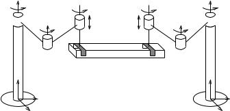
Figure 6.3: Coordinated lifting.

All of the analysis presented here relies on the assumption that the fundamental grasping constraint holds at all times. Even though we are solving for the contact forces, it is important to remember that the contact forces are generated by the constraints. If the contact forces fall outside of the friction cone, then the velocity constraints on the system no longer hold and the equations of motion are no longer given by equation (6.24). It is one of the tasks of control system to keep the contact forces inside the friction cone so that the models we use here remain valid.

2.3Other robot systems

Although the analysis so far has been motivated by grasping, the basic formulation holds for any robot system subject to constraints of the form

with q = (θ, x). Any such system will automatically have dynamics with the same form and structure as those of an open-chain manipulator. In this section, we describe several such examples.

Coordinated lifting

Consider a robotic system which consists of several individual robots lifting a single object, such as the example shown in Figure 6.3. Assume that each robot firmly grasps the object and can exert arbitrary wrenches without losing contact.

To derive the kinematics of this system we can treat each robot as a single finger. The contact model for a robot firmly grasping an object is given by Bci = I Rp×p and F C = Rp. This is just the mathematical statement that the robot can exert arbitrary forces and torques. Substituting these relations into the grasp constraint and identifying the

281

Figure 6.4: The Motoman K10MSB robot performing an arc welding task. (Photograph courtesy of Motoman)

The dynamics of the system follow exactly as in the grasping case.

Workspace dynamics

Many robot systems perform tasks which are most naturally described in workspace coordinates rather than joint space coordinates. For example, in the welding application depicted in Figure 6.4, a natural description of the task would be in terms of the position and orientation of the welding tip. Rather than solve an inverse kinematics problem to generate the corresponding path in joint space, it is possible to directly specify the dynamics in terms of the workspace coordinates (SE(3) for this example).

For simplicity, we work in local coordinates. Let g : Q → Rp represent the forward kinematics of the manipulator and J (θ) = ∂g∂θ the Jacobian. We assume that J is square and nonsingular. We take dynamics of the

282