mls94-complete[1]

becomes

q˙1 = u1 q˙2 = u2

q˙12 = q1u2

q˙121 = q12u1

q˙122 = q12u2.

To steer q1, q2, and q12 to their desired locations, we apply Algorithm 1. To steer q121 independently of the other states, choose u1 = a sin 2πt, u2 = b cos 4πt to obtain

a2b q121(1) = q121(0) − 16π2 .

Similarly, choosing u1 = b cos 4πt, u2 = a sin 2πt gives

a2b q122(1) = q122(0) + 32π2

and all the other states return to their original values.

Both the algorithms presented above require separate steps to steer in each of the qijk directions. It is also possible to generate net motion in multiple coordinates simultaneously by using a linear combination of sinusoids and by solving a polynomial equation for the necessary coe - cients (see Exercise 4).

2.3Higher-order systems: chained form systems

We now study more general examples of nonholonomic systems and investigate the use of sinusoids for steering such systems. As in the previous section, we may try to generate canonical classes of higher order systems, i.e., systems where more than one level of Lie brackets is needed to span the tangent space to the configuration space. Such a development is given by Grayson and Grossmann [37], and in [78] we showed that, in full generality, it is di cult to use sinusoids to steer such systems. This leads us to specialize to a smaller class of higher order systems, which we refer to as chained systems, that can be steered using sinusoids at integrally related frequencies. These systems are interesting in their own right as well, since they are duals of a classical construction in the literature on di erential forms referred to as the Goursat normal form. Further, we can convert many other nonlinear systems into chained form systems as we discuss in the next section.

363

We define the system (8.7) as a one-chain system. The first item is to check the controllability of these systems. To this end, denote iterated Lie products as adkg1 g2, defined by:

adg1 g2 = [g1, g2], adkg1 g2 = [g1, adkg1−1g2] = [g1, [g1, . . . , [g1, g2] . . . ]]

Lemma 8.1. Lie bracket calculations

For the vector fields in equation (8.8), with k ≥ 1

(Here the only non-zero entry is in the (k+2)th entry.)

Proof. By induction. Since the first level of brackets is irregular, we begin

364

by expanding [g1, g2] and [g1, [g1, g2]] to get

Proposition 8.2. Controllability of the one-chain system

The one-chain system (8.7) is completely nonholonomic (controllable).

Proof. There are n coordinates in (8.7) and the n Lie products

{g1, g2, adig1 g2} 1 ≤ i ≤ n − 2

are independent using Lemma 8.1.

To steer this system, we use sinusoids at integrally related frequencies. Roughly speaking, if we use u1 = sin 2πt and u2 = cos 2πkt then q˙3 will have components at frequency 2π(k − 1), q˙4 at frequency 2π(k − 2), etc. q˙k+2 will have a component at frequency zero and when integrated gives motion in qk+2 while all previous variables return to their starting values.

Algorithm 3. Steering chained form systems

1.Steer q1 and q2 to their desired values.

2.For each qk+2, k ≥ 1, steer qk to its final value using u1 = a sin 2πt, u2 = b cos 2πkt, where a and b satisfy

365

Proposition 8.3. Chained form algorithm

Algorithm 3 can steer (8.7) to an arbitrary configuration.

Proof. The proof is constructive. We first show that using u1 = a sin 2πt, u2 = b cos 2πkt produces motion only in qk+2 and not in qj , j < k+2 after one period, by direct integration. If qk−1 has terms at frequency 2πni, then qk has corresponding terms at 2π(ni ±1) (by expanding products of sinusoids as sums of sinusoids). Since the only way to have qi(1) 6= qi(0) is to have qi have a component at frequency zero, it su ces to keep track only of the lowest frequency component in each variable; higher components will integrate to zero. Direct computation starting from the origin yields

1akb t

=2k−1 (2π)kk! 2 + · · ·

the initial conditions generate extra terms of the form qi−1(0)u1 in the ith derivative and this integrates to zero, giving no net contribution.

For the case of systems with more than two inputs, and to the so-called multi-chained form systems, we refer the reader to [78].

3General Methods for Steering

Model control systems of the kind that we discussed in the previous section will very seldom show up verbatim in applications. In this section,

366

we consider some techniques in motion planning for more general nonholonomic systems.

3.1Fourier techniques

The methods involving sinusoids at integrally related frequencies can be modified using some elementary Fourier analysis to steer systems which are not in any of the model classes that we have discussed. We will illustrate these notions on two examples that we studied in Chapter 7.

Example 8.1. Steering the hopping robot in flight

We saw in Chapter 7 that ψ was the angle of the hip of the hopping robot in the flight phase, l the length of the leg extension, and θ the angle of the body of the robot. The control equations are given by

θ = −I + m(l + d)2 u1.

Expanding the right-hand side of the last equation of (8.9) in a Taylor series about l = 0, we get

where O(l2) stands for quadratic and higher-order terms in l. This sug-

α˙ = −(md2 + I)2 lu1 + O(l2)u1 := f (l)u1.

If one neglects the higher order terms in the last equation, this equation has the form of a chained form system with 3 states. Using this as justification, we attempt to use the algorithm for steering chained form systems to steer the precise form of this system. We first steer the ψ and l variables to their desired values. Then, we use sinusoids

u1 = a1 sin 2πt u2 = a2 cos 2πt

to steer α. By choice, after one period (1 second), the last motion does not a ect the final values of ψ and l. Since l = 2aπ2 sin 2πt over this piece

367

of the motion, we can expand f (l) by its Fourier series as f ( 2aπ2 sin 2πt) = β1 sin 2πt + β2 sin 4πt + · · ·

Integrating α˙ over one period and noting that only the first term contributes to the net motion, yields

Z 1

α(1) − α(0) = (a1β1 sin2 2πt + a1β2 sin 2πt sin 4πt + · · · ) dt

0

1

= 2 a1β1.

Since β1 is a function of a2, one can solve for a1, a2 numerically to achieve a net change in α. Cartwheeling in mid-air consists of a net change in phase of 2π radians.

Example 8.2. Steering the kinematic car

The equations for the kinematic model of a front wheel drive car are given by (7.14), namely

x˙ = cos θ u1 y˙ = sin θ u1

˙

φ = u2.

In this form, u1 does not control any state directly. We use a change of coordinates z1 = x, z2 = φ, z3 = sin θ, z4 = y, and a change of inputs v1 = cos θ u1, v2 = u2 to put the equations in the form

sions of the nonlinearities in the last two equations match the terms of the one-chain system, and we can include the e ect of the nonlinear terms using Fourier analysis.

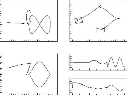
An example of the application of Algorithm 2 applied to the car is given in Figure 8.1. The first part of the path, labeled A, drives x and φ to their desired values using a constant input. The second portion labeled B, uses a sine and cosine to drive θ while bringing the other two states back to their desired values. The last step labeled C, involving the inputs

u1 = a1 sin 4πt u2 = a2 sin 2πt,

368

Figure 8.1: Sample trajectories for the motion of a car. The trajectory shown is a sample path which moves the car from (x, y, θ, φ) = (−5, 1, 0.05, 1) to (0, 0.5, 0, 0). The first three figures show the states versus x, the bottom right graphs show the inputs as functions of time.

brings y to the desired value and returns the other states back to their correct values. The Lissajous figures obtained from the phase portraits of the di erent variables are quite instructive. Consider the part of the curve labeled C. The upper left plot contains the Lissajous figure for x, φ (two loops); the lower left plot is the corresponding figure for x, θ (one loop); and the open curve in x, y shows the increment in the y variable. The interesting implication here is that the Lie bracket motions correspond to rectification of harmonic periodic motions of the driving vector fields, and the harmonic relations are determined by the order of the Lie bracket corresponding to the desired direction of motion.

3.2Conversion to chained form

An interesting question to ask is whether it is possible using a change of input and nonlinear transformation of the coordinates to convert a given nonholonomic control system into one of the model forms discussed in

369

the previous section. More precisely, given the system

q˙ = g1(q)u1 + · · · + gm(q)um,

does there exist a matrix β(q) Rm×m and a di eomorphism φ : Rn → Rn such that with

v = β(q)u z = φ(q),

the system is in chained form in the z coordinates with inputs v? One can give necessary and su cient conditions to solve this problem (see [74]), but the discussion of these conditions would take us into far too much detail for this section. In [78], we gave su cient conditions for the two-input case, in which case the system was to be converted into the onechain form. The conditions assume that g1, g2 are linearly independent. Now, the system can be converted into one-chain form if the following distributions are all of constant rank and involutive:

0 = span{g1, g2, adg1 g2, . . . , adng1−2 g1}

1 = span{g2, adg1 g2, . . . , adng1−2 g2} 2 = span{g2, adg1 g2, . . . , adng1−3 g2}

and there exists a function h1(q) such that

dh1 · 1 = 0 and dh1 · g1 = 1.

If these conditions are met, then a function h2 independent of h1 may be chosen so that

dh2 · 2 = 0.

The existence of independent h1 and h2 so that dh1 · 1 = 0, dh2 · 2 = 0 is guaranteed by Frobenius’ theorem, since 2 1 are both involutive distributions. There is however an added condition on h1, namely that dh1 ·g1 = 1. If we can find these functions h1, h2, then the map φ : q 7→z and input transformation given by

370

This procedure can be illustrated on the kinematic model of a car.

Example 8.3. Conversion of the kinematic car into chained form

First, we rewrite the kinematic equations as

˙

φ = u2.

Then, with h1 = x and h2 = y, it is easy to verify that this system satisfies the conditions given above and the change of variables and input are given by

to give a one-chain system.

3.3Optimal steering of nonholonomic systems

In this section, we discuss the least squares optimal control problem for steering a control system of the form

q˙ = g1(q)u1 + · · · + gm(q)um

from q0 to qf in 1 second. Thus, we minimize the cost function

1 Z 1 ku(t)k2 dt.

2 0

Our treatment here is, of necessity, somewhat informal; to get all the smoothness hypotheses worked out would be far too large an excursion to make here. We will assume that the steering problem has a solution (by Chow’s theorem, this is guaranteed when the controllability Lie algebra generated by g1, . . . , gm is of rank n for all q). We give a heuristic derivation from the calculus of variations of the necessary conditions for optimality. To do so, we incorporate the constraints into the cost function using a Lagrange multiplier function p(t) Rn to get

371

Introduce the Hamiltonian function:

Using this definition and integrating the second term of (8.10) by parts

Consider the variation in J caused by variations in the control input u,1

If the optimal input has been found, a necessary condition for stationarity is that the first variation above be zero for all variations δu and δq:

From the second of these equations, it follows that the optimal inputs are given by

with boundary conditions q(0) = q0 and q(1) = qf . Using this result, we may derive the following proposition about the structure of the optimal controls:

Proposition 8.4. Constant norm of optimal controls

For the least squares optimal control problem for the control system

m

X

q˙ = gi(q)ui

i=1

1In the calculus of variations, one makes a variation in u, namely δu, and calculates the changes in the quantities p and H as δp and δH. See for example [123].

372