

mls94-complete[1]
.pdftransport. Furthermore, custom end-e ectors are capable of generating stable and rigid grasps by design; a similar grasp using an articulated hand requires the use of feedback control and results in an overall decrease in the rigidity of the grasp. Nonetheless, for many situations, a multifingered robot hand attached to a robot arm is an attractive solution to a di cult problem. The principles involved in the study of robot hands are applicable to a number of other areas, most notably coordinated manipulation between robots. Indeed, if we view two (large) robots as fingers of a hand, then the problem of coordinated lifting reduces to a problem in grasping. With this point of view in mind, we will present the study of multifingered hands in a framework which is applicable to a large class of robot systems.
Overview
We break the study of multifingered robot hands into two basic parts: kinematics and planning, and dynamics and control. In each of these areas, the techniques presented in previous chapters are extended to account for the additional complexity of a robot hand. We will also see many new techniques which are unique to the study of multifingered hands, such as grasp planning and the kinematics of rolling contact.
We begin with a detailed study of the kinematics of a multifingered robot hand. Given models of an object, a set of robot fingers, and the contact between the fingers and the object, we wish to find the relationship between forces and motions of the object and fingers. We will be interested primarily with the kinematics of this system when the fingers do not slip on the object. An implicit assumption in studying the kinematics of the hand is that the contact locations are known (or can be measured). Under this assumption, we compute the fundamental grasping constraint which governs the motion of the hand.
The grasp planning problem is to determine a set of contact locations for the object and the fingers. To do so, we first characterize desirable properties of a grasp. These properties include:
1.The ability to resist external forces. Given a wrench applied to an object, we wish to apply contact forces which generate an opposing wrench. We will refer to a grasp in which the fingers can resist arbitrary external forces as a force-closure grasp.
2.The ability to dextrously manipulate the object. In order to manipulate an object, we must be able to move the object in a way compatible with the desired task. Depending on the task, this may require independent motion in all directions or only some directions. We refer to a grasp in which the fingers can accommodate arbitrary object motions as a manipulable grasp.
213
Given an object, we seek to choose contacts so that these properties hold wherever possible. We will briefly present some procedures for choosing the locations of the contacts for some simple cases which illustrate the techniques available.
Chapter 6 studies the dynamics and control problem for multifingered robot hands. We extend the dynamic formulation presented in Chapter 4 to include robotic systems with contact constraints. In fact, it is possible to do so in such a way that all of the control laws which can be applied to robot manipulators can be immediately extended and applied to multifingered robot hands. We also present extensions for dynamics and control of redundant robots, as these are often present in multifingered robot systems.
Throughout this chapter and the next, we make two assumptions to allow precise analysis:
1.The object is a rigid body in contact with a rigid link robot.
2.Accurate models of the fingers and object are given.
The relaxation of these conditions is a topic of current research (see, for example, [47, 73]).
2Grasp Statics
We begin by studying a particularly simple case in which all contacts between the fingers and the object are idealized as point contacts at a fixed location. This case allows one to ignore the possibility that a finger rolls or slides along the surface of the object (a possibility which we shall study in some detail later). We also begin by ignoring the kinematics of the fingers which make up the hand: we consider only the transmission of forces between a set of contacts and the object.
2.1Contact models
A contact between a finger and an object can be described as a mapping between forces exerted by the finger at the point of contact and the resultant wrenches at some reference point on the object. In order to simplify the formulation of the dynamics in Chapter 6, we always choose the object reference point to be the center of mass of the object. We represent the forces at the contacts and on the object in terms of a set of coordinate frames attached at each contact location and the object reference point. We assume that the location of the contact point on the object is fixed.
For convenience, we shall always choose the contact coordinate frame, Ci, such that the z-axis of this frame points in the direction of the inward
214
|
z |
x |
Ci |
|
|
|
|
|
y |
z |
y |
|
|
||
z |
O |
|
|
|
|
|
|
|
x |
|
|
|
|
goci |
|
 y
y
P
gpo
x
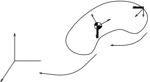
Figure 5.2: Coordinate frames for contact and object forces.
surface normal at the point of contact (as shown in Figure 5.2). We describe the contact location by its relative position and orientation with respect to the object reference frame, O. That is,
goci = (poci , Roci ) SE(3)
is the location of the contact with respect to the object. The action of goci is to take the coordinates of a point given in the contact coordinate frame and return the coordinates of the same point in the object coordinate frame. The configuration of the object relative to a fixed palm frame is given by xo := gpo SE(3). The force applied by a contact is modeled as a wrench Fci applied at the origin of the contact frame, Ci.
Typically, a finger will not be able to exert forces in every direction; several simple contact models are used to classify common contact configurations. We begin by studying the simplest of these contact types: one in which the finger is only allowed to apply normal forces to the object at the contact location. We then extend this analysis to include some simple models of friction.
A frictionless point contact is obtained when there is no friction between the fingertip and the object. In this case, forces can only be applied in the direction normal to the surface of the object and hence we can represent the applied wrench as
0
0
|
|
0 |
|
|
|
|
|
Fci = |
|
1 |
|
fci fci |
≥ |
0, |
(5.1) |
|
0 |
|
|||||
|
0 |
|
|
where fci R is the magnitude of the force applied by the finger in the normal direction. The requirement that fci be positive models the fact that a contact of this type can push on an object, but it cannot pull on the object.
215
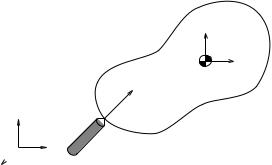
 O
O
Fci
 P
P
Figure 5.3: Frictionless point contact.
Frictionless point contacts almost never occur in a practical situation, but they can serve as a useful model for contacts in which the friction between the finger and the object is low or unknown. Since a frictionless contact cannot exert forces except in the normal direction, modeling a contact as frictionless insures that we do not rely on frictional forces when we manipulate the object.
For grasps in which we do wish to make use of frictional forces, we must provide a model for friction. We will use a simple model which is often referred to as the Coulomb friction model. We would like to describe how much force a contact can apply in the tangent directions to a surface as a function of the applied normal force. The Coulomb friction model is an empirical model which asserts that the allowed tangential force is proportional to the applied normal force, and the constant of proportionality is a function of the materials which are in contact.
If we let f t R denote the magnitude of the tangential force and f n R denote the magnitude of the normal force, Coulomb’s law states
that slipping begins when
|f t| > µf n,
where µ > 0 is the (static) coe cient of friction. This implies that the range of tangential forces which can be applied at a contact is given by
|f t| ≤ µf n. |
(5.2) |
In particular, we see that f n must be positive in order for this relationship to hold for at least some non-zero f t.
Equation (5.2) can be represented geometrically, as shown in Figure 5.4. The set of forces which can be applied at a contact must lie in a cone centered about the surface normal. This cone is called the friction cone; the angle of the cone with respect to the normal is given by
α = tan−1 µ.
216
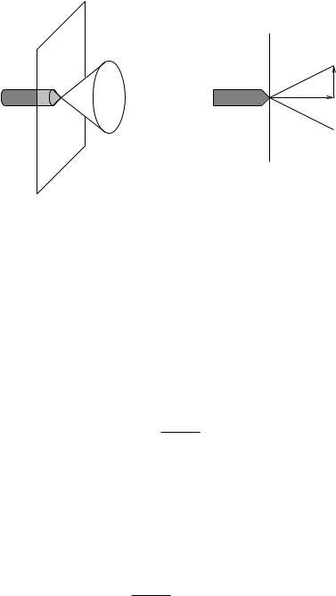
friction
cone
fn µfn
 α
α
object surface
side view
Figure 5.4: Geometric interpretation of the Coulomb friction model.
A short table of friction coe cients for common materials is given in Table 5.1. Typical values of µ are less than 1, and hence the friction cone angle is typically less than 45◦.
A point contact with friction model is used when friction exists between the fingertip and the object, in which case forces can be exerted in any direction that is within the friction cone for the contact. We represent the wrench applied to the object with respect to a basis of directions which are consistent with the friction model:
1 0 0
0 1 0
|
|
0 0 0 |
|
|
|
|
|
|
Fci = |
|
0 0 1 |
|
fci |
fci |
|
F Cci , |
(5.3) |
|
0 0 0 |
|
||||||
|
|
0 0 0 |
|
|
|
|
|
where q
F Cci = {f R3 : f12 + f22 ≤ µf3, f3 ≥ 0}.
A more realistic contact model is the soft-finger contact. Here we allow not only forces to be applied in a cone about the surface normal, but also torques about that normal. For simplicity, we model the torques as being limited by a torsional friction coe cient. The applied contact wrench is
Fci = |
1 0 0 0 |
fci |
|
|
|
|
0 1 0 0 |
|
|
|
|
||
0 0 1 0 |
fci |
|
F Cci |
(5.4) |
||
0 0 0 0 |
||||||
|
0 0 0 0 |
|
|
|
|
|
0 0 0 1 |
|
|
|
|
and the friction cone becomes q
F Cci = {f R4 : f12 + f22 ≤ µf3, f3 ≥ 0, |f4| ≤ γf3},
where γ > 0 is the coe cient of torsional friction.
217
Table 5.1: Static friction coe cients for some common materials. (Source: CRC Handbook of Chemistry and Physics)
|
Steel on steel |
0.58 |
Wood on wood |
0.25-0.5 |
|
Polyethylene on steel |
0.3–0.35 |
Wood on metals |
0.2-0.6 |
|
Polyethylene on self |
0.5 |
Wood on leather |
0.3–0.4 |
|
Rubber on solids |
1–4 |
Leather on metal |
0.6 |
|
|
|
|
|
In general, we model a contact using a wrench basis, Bci Rp×mi , and a friction cone, F Cci . In all of our examples, we chose p = 6, the dimension of the space of generalized forces that can be applied in SE(3). Other choices are possible, the most common being p = 3, which is used for planar grasping. The dimension of the wrench basis, mi, indicates the number of independent forces that can be applied by the contact. We require that F Cci satisfy the following properties:
1. F Cci is a closed subset of Rmi with non-empty interior.
2. f1, f2 F Cci = αf1 + βf2 F Cci for α, β > 0.
The set of allowable contact forces applied by a given contact is:
Fci = Bci fci fci F Cci . |
(5.5) |
Several common contact types are summarized in Table 5.2. Other contacts, such as line and face contacts, are explored in the exercises.
2.2The grasp map
To determine the e ect of the contact forces on the object, we transform the forces to the object coordinate frame. Let (poci , Roci ) be the configuration of the ith contact frame relative to the object frame. Then, the force exerted by a single contact can be written in object coordinates as
Fo = Adgoc− i |
Fci |
= |
poci Roci |
Roci Bci fci , |
fci F Cci . |
T |
|
|
Roci |
0 |
|
1 |
is thebwrench transformation matrix which maps |
||||
T |
|||||
The matrix Adgoc−1 |
|||||
i |
|
|
|
|
|
contact wrenches to object wrenches. For brevity we shall often write (pci , Rci ) for the configuration of the ith contact frame, dropping the o subscript. We define the contact map, Gi Rp×mi , to be the linear map between contact forces, represented with respect to Bci , and the object wrench:
Gi := AdT−1 Bci .
goci
218
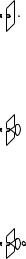
Table 5.2: Common contact types.
|
Contact type |
|
|
Picture |
Wrench basis |
|
|
FC |
|||||||||||
|
|
|
|
|
|
|
|
|
|
|
|
|
|
|
|
|
|
||
|
|
|
|
|
|
|
|
|
|
0 |
|
|
|
|
|
|
|
||
|
|
|
|
|
|
|
|
|
|
|
0 |
|
|
|
|
|
|
|
|
|
|
|
|
|
|
|
|
|
|
|
|
|
|
|
|
|
|
|
|
|
Frictionless |
|
|
|
|
|
|
|
|
0 |
|
|
|
|
|
|
|
||
|
|
|
|
|
|
|
|
|
|
|
|
|
|
|
|
|
|
|
|
|
point contact |
|
|
|
|
|
|
|
|
0 |
|
|
|
|
|
|
|
||
|
|
|
|
|
|
|
|
|
0 |
|
|
|
|
|
f1 ≥ 0 |
||||
|
|
|
|
|
|
|
|
|
|
|
|
|
|
|
|
|
|
|
|
|
|
|
|
|
|
|
|
|
|
|
|
|
|
|
|
|
|
|
|
|
|
|
|
|
|
|
|
0 |
|
1 |
|
0 |
|
|
|
|
|
||
|
|
|
|
|
|
|
|
|
1 |
|
0 |
|
0 |
|
|
|
|
|
|
|
|
|
|
|
|
|
|
|
|
|
0 |
|
|
|
|
|
|
|
|
|
Point contact |
|
|
|
|
|
|
0 |
|
|
0 |
|
|
|
|
|
|||
|
|
|
|
|
|
|
|
0 |
|
0 |
|
1 |
|
|
p |
f 2 + f22 ≤ µf3 |
|||
|
with friction |
|
|
|
|
|
|
0 |
|
0 |
|
0 |
|
|
|
|
|||
|
|
|
|
|
|
|
0 |
|
0 |
|
0 |
|
1 |
f3 ≥ 0 |
|||||
|
|
|
|
|
|
|
|
|
|
|
|
|
|
|
|
|
|
|
|
|
|
|
|
|
|
|
|
|
|
|
|
|
|
|
|
|
|
|
|
|
|
|
|
|
|
|
|
1 |
|
0 |
|
0 |
|
0 |
|
|
|
|
|
|
|
|
|
|
|
|
0 1 |
|
0 0 |
|
|
||||||||
|
|
|
|
|
|
|
|
|
|
|
|
||||||||
|
|
|
|
|
|
|
|
|
|
||||||||||
|
|
|
|
|
|
|
|
|
|
|
|||||||||
|
|
|
|
|
|
|
|
p |
f12 + f22 ≤ µf3 |
||||||||||
|
|
|
|
|
|
|
0 |
|
0 |
|
0 |
|
0 |
|
|
|
|||
|
Soft-finger |
|
|
|
|
|
|
0 |
|
0 |
|
1 |
|
0 |
|
|
f3 ≥ 0 |
||
|
|
|
|
|
|
0 |
|
0 |
|
0 |
|
0 |
|
||||||
|
|
|
|
|
|
|
0 |
|
0 |
|
0 |
|
1 |
|
|
|
|
||
|
|
|
|
|
|
|
|
|
|
|
|
|
|
|
|
|
|f4| ≤ γf3 |
||
|
|
|
|
|
|
|
|
|
|
|
|
|
|
|
|
|
|||
|
|
|
|
|
|
|
|
|
|
|
|
|
|
|
|
|
|
|
|
If we have k fingers contacting an object, the total wrench on the object is the sum of the object wrenches due to each finger. The map between the contact forces and the total object force is called the grasp map, G : Rm → Rp, m = m1 + · · · + mk. Since each contact map is linear and wrenches can be superposed (as long as they are all written in the same coordinate frame), the net object wrench is
Fo = G1fc1 + + Gkfck |
= G1 |
|
Gk |
.. |
|
, |
||||||||
|
|
· · · |
|
|
|
|
|
· · · |
|
|
|
fc1 |
|
|
|
|
|
|
|
|
|
fck |
|
||||||
|
|
|
|
|
|
|
|
|
|
|
. |
|
|
|
and the grasp map is |
|
|
|
|
|
|
|
|
|
|
||||
|
|
|
|
|
|
|
|
|
|
|
|
|
||
|
|
|
|
|
|
|
|
|
|
|
|
|
|
|
|
|
T |
1 |
Bc1 |
· · · |
|
T |
Bck i |
|
|
|
(5.6) |
||
|
G = hAdgoc− |
Adgoc− k |
|
|
|
|||||||||
|
|
|
1 |
|
|
|
1 |
|
|
|
|
|
|
|
With this definition, the object wrench can be written
Fo = Gfc |
fc F C, |
(5.7) |
219
where
fc = (fc1 , . . . , fck ) Rm
F C = F Cc1 × · · · × F Cck Rm m = m1 + · · · + mk.
Thus, a grasp is completely described by the grasp map G and the friction cone F C.
Definition 5.1. Representation of a grasp
A complete description of a grasp consists of a matrix G Rp×m and a set F C Rm which satisfies the following properties:
1. F C is a closed subset of Rm with non-empty interior.
2. f1, f2 F C = αf1 + βf2 F C for α, β > 0.
The set of wrenches that can be applied to the object by the contacts has the form
Fo = Gfc |
fc F C. |
From now on, we will represent a grasp by the quantities G and F C. We often omit explicit mention of the friction cone and refer to G as a grasp.
Example 5.1. Grasp map for frictionless point contacts
Consider first the case of several point contacts touching an object. Then, each contact wrench can be written as
Fo = |
pci Rci |
Rci |
|
|
0 |
fci fci |
≥ |
0. |
|
|
|
|
|
|
0 |
|
|
||
|
|
|
|
|
|
0 |
|
|
|
|
Rci |
0 |
|
|
0 |
|
|
|
|
|
|
1 |
|
|
|||||
|
|
|
|
0 |
|
|
|||
Performing the matrix multiplication,b |
we see that the object wrench has |
||||||||
the form |
Fo = |
pci |
×inci fci |
|
|
||||
|
|
|
nc |
|
|
|
|
|
|
where nci is the direction of the inward surface normal written in the object coordinate frame. Combining the e ect of each of the fingers yields:
Fo = |
|
· · · |
|
|
.. |
|
= Gfc, |
|
|
|
|
pc1 |
× nc1 |
· · · |
pck |
× nck |
|
fc1 |
|
fci |
≥ 0. |
||
fck |
|
||||||||||
|
nc1 |
|
|
nck |
|
. |
|
|
Fo |
|
R6 |
|
|
|
|
|
|
|
|
|
|
||
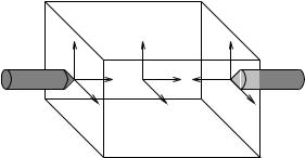
Example 5.2. Soft-finger grasp of a box
Consider a box grasped by two soft-finger contacts, as shown in Figure 5.5. The position of the contact frame with respect to the object
220
x |
z |
y |
|
z |
y z |
y |
x |
x |
Figure 5.5: Box grasped by two fingers.
frame is given by |
|
|
−r |
|
|
0 |
|
−1 |
|
|
r . |
||||
Rc1 |
= |
0 |
0 |
1 |
pc1 |
= |
Rc2 |
= |
0 |
pc2 |
= |
||||
|
|
0 |
1 |
0 |
|
|
0 |
|
|
1 |
0 |
0 |
|
|
0 |
|
|
1 |
0 |
0 |
|
|
0 |
|
|
0 |
1 |
0 |
|
|
0 |
The grasp map for each finger is obtained by transforming the standard wrench basis into the object coordinate frame:
Gi = pc Rc |
Rc |
|
0 0 0 0 . |
||||
|
|
|
|
i |
|
1 0 0 0 |
|
|
Rci |
0 |
|
0 1 0 0 |
|
||
b |
0 0 1 0 |
||||||
|
|
0 0 0 1 |
|||||
|
i i |
|
|
0 0 0 0 |
|
||
Calculating and combining these gives the grasp map,
|
|
0 |
0 |
1 |
0 |
|
0 |
−1 |
0 |
|
|
|||
|
0 |
|
||||||||||||
|
|
0 |
1 |
0 |
0 |
1 |
0 |
0 |
0 |
|
|
|||
G = |
|
r 0 |
0 |
0 |
0 |
+r |
0 |
0 |
, |
|||||
|
|
|
|
|
|
|
|
|
|
|
|
|
|
|
|
− |
|
0 |
0 |
1 |
0 |
0 |
0 |
|
1 |
|
|||
|
|
0 |
|
|
|
|||||||||
|
|
1 |
0 |
0 |
0 |
0 |
1 |
0 |
0 |
|
|
|||
|
0 |
+r |
0 |
0 |
|
r |
0 |
0 |
− |
|
|
|||
|
|
|
0 |
|
|
|||||||||
|
|
|
|
|
|
|
|
|
|
|
|
|
|
|
|
|
|
|
|
|
|
− |
|
|
|
|
|
|
|
with contact forces
|
fc = (fc11 , fc21 , fc31 , fc41 , fc12 , fc22 , fc32 , fc42 ) R8. |
||
The friction cone in this coordinate frame is given by: |
|||
F C = F Cc1 × F Cc2 |
|||
|
= nfc : q |
|
≤ µfc31 , |fc41 | ≤ γfc31 , fc31 ≥ 0o |
F Cc1 |
(fc11 )2 + (fc21 )2 |
||
|
= nfc : q |
|
≤ µfc32 , |fc42 | ≤ γfc32 , fc32 ≥ 0o . |
F Cc2 |
(fc12 )2 + (fc22 )2 |
||
221
|
2r |
|
|
y |
x |
|
y |
y |
|
O |
x |
|
|
|
C1 |
x |
C2 |
|
|
|
|
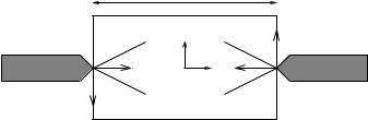
Figure 5.6: Planar grasping. |
|
Example 5.3. Planar grasp of a rectangle
Consider the planar grasp shown in Figure 5.6. Rather than analyze this grasp in SE(3), we specialize our results to SE(2). A wrench in SE(2) is represented by a linear component f R2 and an angular component τ R. f corresponds to the forces in the plane and τ to the torque about the normal to the plane (see Exercise 2.11). Wrenches in SE(2)
are transformed by the rule |
−py |
|
|
|
|
|
|
1 τci |
|
|
τo = |
|
px |
Rci |
, |
||||||
fo |
|
Rci |
|
|
|
0 |
fci |
|
||
where Rci SO(2) and pci |
= (p |
|
, p |
|
) |
|
R2 |
|
|
|
|
x |
|
y |
|
|
represents the location of ci |
||||
relative to the object reference frame.
Given these definitions, we can proceed to analyze Figure 5.6. In SE(2), we shall choose contact coordinate frames such that the y-axis points in the direction of the inward surface normal. With this choice,
the contact locations are |
|
|
|
|
1 0 |
|
|
|
|||
|
1 |
−1 0 |
|
2 |
|
|
|||||
Rc |
|
= |
0 1 |
Rc |
|
= 0 |
−1 |
|
|
||
|
1 |
|
0 |
|
|
2 |
0 |
|
|
|
|
pc |
|
= −r |
|
pc |
|
= r . |
|
|
|
|
|
A wrench basis for a point contact with friction is |
|
|
|
||||||||
|
|
|
Bci = 0 |
1 |
|
|
|
|
|||
|
|
|
|
1 |
0 |
|
|
|
|
|
|
|
|
|
|
0 |
0 |
|
|
|
|
||
with the friction cone constraint written as |
|
|
|
|
|||||||
fci |
F Cci |
|
|
|
|
|
|
|
|||
F Cci = {f R2 : |f1| ≤ µf2, f2 ≥ 0}. |
|
|
|||||||||
Finally, the grasp map is given by |
|
|
−1 |
|
|
|
. |
||||
G = Adgoc− 1 |
Bc1 |
Adgoc− 2 Bc2 = |
0 1 0 |
||||||||
T |
|
|
|
T |
i |
|
0 |
1 |
0 |
−1 |
|
h |
|
|
|
1 |
|
r |
0 |
r |
0 |
|
|
1 |
|
|
|
|
|
|
|
|
|
||
222