mls94-complete[1]

Figure 3.10: Subproblem 3: (a) Rotate p about the axis of ξ until it is a distance δ from q. (b) The projection onto the plane perpendicular to the axis. The dashed line is the “flip” solution.

We can also “project” δ by subtracting the component of p − q in the ω direction,

δ′2 = δ2 − |ωT (p − q)|2,

so that equation (3.27) becomes

kv′ − eωθb u′k2 = δ′2

(see Figure 3.10b). If we let θ0 be the angle between the vectors u′ and v′, we have

We can now use the law of cosines to solve for the angle φ = θ0 − θ. The triangle formed by the center of the axis, exp(ωθb )u′, and v′ satisfies

ku′k2 + kv′k2 − 2ku′kkv′k cos φ = δ′2

Equation (3.29) has either zero, one, or two solutions, depending on the

number of points in which the circle of radius ku′k intersects the circle of radius δ′.

103

3.3Solving inverse kinematics using subproblems

Given the solutions to the subproblems presented above, we must now find techniques for converting the complete inverse kinematics problem into the appropriate subproblems.

The basic technique for simplification is to apply the kinematic equations to special points, such as the intersection of two or more axes. This

b

is a potentially powerful operation since exp(ξθ)p = p if p is on the axis of a revolute twist ξ. Using this, we can eliminate the dependence of certain joint angles by appropriate selection of points. For example, if we wish to solve

with ξ1, ξ2, and ξ3 all zero-pitch twists, then applying both sides to a point p on the axis of ξ3 yields

b b

eξ1θ1 eξ2θ2 p = gp,

which can be solved using Subproblem 2 (in the case that ξ1 and ξ2 intersect).

Another common trick for reducing a problem to a subproblem is to subtract a point from both sides of an equation and take the norm of the result. Since rigid motions preserve norm, some dependencies can be eliminated. For example, if we wish to solve

for ξ3, and ξ1, ξ2 intersect at a point q, then we can apply both sides of the equation to a point p that is not on the axis of ξ3 and subtract the point q. Taking the norm of the result yields

which is Subproblem 3.

We now show how the subproblems of Section 3.2 can be used to solve the inverse kinematics of some common manipulators. Additional examples appear in the exercises.

Example 3.5. Elbow manipulator inverse kinematics

The elbow manipulator in Figure 3.11 consists of a three degree of freedom manipulator with a spherical wrist. This special structure simplifies the inverse kinematics and fits nicely with the subproblems presented earlier.

The equation we wish to solve is

104

l0

S

Figure 3.11: Elbow manipulator.

where gd SE(3) is the desired configuration of the tool frame. Postmultiplying this equation by gst−1(0) isolates the exponential maps:

We determine the requisite joint angles in four steps.

Step 1 (solve for the elbow angle, θ3). Apply both sides of equation (3.30) to a point pw R3 which is the common point of intersection for the wrist axes. Since exp(ξθ)p = pw if pw is on the axis of ξ, this yields

Subtract from both sides of equation (3.31) a point pb which is at the intersection of the first two axes, as shown in Figure 3.11:

Using the property that the distance between points is preserved by rigid motions, take the magnitude of both sides of equation (3.32):

This equation is in the form required for Subproblem 3, with p = pw , q = pb, and δ = kg1pw − pbk. Applying Subproblem 3, we solve for θ3.

Step 2 (solve for the base joint angles). Since θ3 is known, equation (3.31) becomes

b

Applying Subproblem 2 with p = exp(ξ3θ3)pw and q = g1pw gives the values for θ1 and θ2.

105

Step 3 (solve for two of three wrist angles). The remaining kinematics can be written as

Apply both sides of equation (3.35) to a point p which is on the axis of ξ6 but not on the ξ4, ξ5 axes. This gives

Apply Subproblem 2 to find θ4 and θ5.

Step 4 (solve for the remaining wrist angle). The only remaining unknown is θ6. Rearranging the kinematics equation and applying both sides to any point p which is not on the axis of ξ6,

Apply Subproblem 1 to find θ6.

At the end of this procedure, θ1 through θ6 are determined. There are a maximum of eight possible solutions, due to multiple solutions for equations (3.33), (3.34), and (3.36). Note that the overall procedure is to first solve for the three angles which determine the position of the center of the wrist and then solve for the wrist angles.

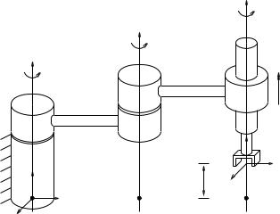
Example 3.6. Inverse kinematics of a SCARA manipulator

Consider the four degree of freedom SCARA manipulator shown in Figure 3.12. From the forward kinematics derived in Example 3.1 on page 87, the tool configuration has the form

(3.38) and hence we can solve the inverse kinematics given x, y, z, and φ as in equation (3.38). We begin by solving for θ4. Applying both sides of equation (3.38) to the origin of the tool frame gives

where p(θ) is the position component of the forward kinematics, given by equation (3.4). From the form of p(θ), we see that θ4 = z −l0. Notice that finding θ4 did not make use of any of the previously defined subproblems.

106

x

Figure 3.12: SCARA manipulator in its reference configuration.

Once θ4 is known, we can rearrange equation (3.38) to read

Let p be a point on the axis of ξ3 and q be a point on the axis of ξ1. Applying equation (3.39) to p, subtracting q from both sides, and applying norms,

b

(3.40)

= keξ2θ2 p − qk = kg1p − qk =: δ.

Application of Subproblem 3 gives the value of θ2. θ1 can now be found by applying equation (3.39) to a point p′ on the axis of ξ3 and solving Subproblem 1:

Finally, we rearrange equation (3.39), shifting the (known) θ1 and θ2 terms to the right-hand side:

Applying equation (3.41) to any point p which is not on the axis of ξ3 and solving Subproblem 1 a final time gives θ3 and completes the solution.

There are a maximum of two possible solutions for the SCARA manipulator, corresponding to the solutions of equation (3.40).

107

3.4General solutions to inverse kinematics problems

In the preceding sections, we have developed an elegant set of geometric and conceptual subproblems in terms of which the inverse kinematics solution of a large number of manipulators can be decomposed. The set of subproblems and their extensions given in the exercises turn out to be useful for decomposing the solution of the inverse kinematics equations, primarily when the robot has at least some intersecting axes.

The question of how to solve the inverse kinematics problem in general, (that is, in the absence of any intersections of the axes of the manipulator) for both planar and spatial mechanisms is an extremely active area of current research. In particular, there are many interesting questions about the number of inverse kinematics solutions and how the computations can be mechanized in real-time. In this subsection, we give a brief summary of some of the newest and most general approaches in this regard, drawn from [57], [64] and [95]. Our development closely parallels that of Manocha and Canny [64]. The approaches are primarily based on classic elimination theory from algebraic geometry; this is a systematic procedure for simultaneously eliminating n − 1 of the variables in a system of n polynomials in n variables to obtain a single polynomial in one variable. This procedure is a general procedure but also a “brute-force” procedure, in that it only takes very simple properties of the manipulator kinematics into account (unlike the solutions based on the subproblems listed above). We illustrate this procedure, sometimes referred to as dialytical elimination, in the following example of three nonhomogeneous polynomials in three variables.

Example 3.7. Dialytical elimination for three polynomials in three variables

We will assume that the three polynomials f1, f2, f3 are nonhomogeneous in x1, x2, x3 and are of the form

Here, ai, bi, ci, di, ei, gi, for i = 1, . . . , 3 are all real numbers. To solve this system of three polynomials in x1, x2, x3 for their common zeros, we eliminate x2, x3 to get a single polynomial in x1 in two steps:

Step 1. We express the above equation as a system of equations in x2, x3

108

Step 2. We try to generate more polynomials which are independent2 of f1, f2, f3 until we have as many unknown monomials3 in x2, x3 as there are equations. For example, multiplying f1, f2, f3 by x2 yields the following set of polynomials which are independent of f1, f2, f3:

Combining these equations with those for f1, f2, f3 yields the following set of six equations in the six monomials x32, x22, x2x3, x2, x3, 1:

For this equation to have a solution, it is clear that the determinant of the matrix A(x1) multiplying the entries x32, x2x3, x22, x2, x3, 1 should have zero determinant. Thus, the system of equations f1 = f2 = f3 = 0 is equivalent to det A(x1) = 0. In general, the degree of this polynomial in x1 is high (generically, i.e., for almost all values of ai, . . . , gi, its degree is six) and, furthermore, solutions need not be real. However, the degree of the polynomial is an upper bound on the number of real solutions and once a real number x1 has been found, one can read o the solution for x2, x3 by scaling the element in the null space of A(x1) to have 1 as its last entry. If the null space of the matrix A(x1) has dimension greater than one, corresponding to a multiplicity of roots for the polynomial det A(x1) = 0, then there may be a multiplicity of solutions for x2, x3 corresponding to the value(s) of x1 for which the null space of the matrix A(x1) has dimension greater than 1. While the exact multiplicity is a subtle question in [64], it is stated that an upper bound for the multiplicity of the solutions x2, x3 associated with that value of x1 is the dimension of the null space of A(x1).

2Independence is meant in a technical sense, over the ring of polynomials in x1. 3A monomial is a single polynomial; for example, x2x3 or x31.

109

A general procedure for six degree of freedom manipulators

To apply this procedure to the inverse kinematics of a six-link manipulator, some preliminary work is necessary. The kinematics are given by

and the inverse kinematics problem is to solve for θ1, . . . , θ6 given gd SE(3). We rewrite the kinematics in terms of the Denavit-Hartenberg parameterization, as in equation (3.6):

(3.42) Given a desired gd for the end-e ector position and orientation, we rewrite this equation as

What we have done is to take the inverses of gl5l6 (θ6), gl0l1 (θ1), and gl1l2 (θ2) and moved them to the right-hand side. The reason for this clever rearrangement and the choice of the Denavit-Hartenberg parameterization in the kinematics will become clear in Step 1 of the procedure

which follows. By way of notation, we write gdg−1 as

l6t

Hence, l, m, n R3 are the columns of the rotational component of gdg−1

l6t

and and q R3 is the translational component.

To bring to bear the machinery of algebraic geometry in an equation involving sines and cosines of angles, we define ci := cos θi and si := sin θi for i = 1, . . . , 6 and think of equation (3.43) as being polynomial in si and ci. Indeed, by direct inspection we may see that the entries of each exponential are unary (i.e., of degree 1 or less) in ci and si. Part of the reason for rewriting the kinematics as in equation (3.43) is to be able to reduce the order of the polynomial in si and ci. Both the left-hand side and right-hand side of (3.43) are now cubic in si and ci. The details of the procedure to eliminate all the variables except for θ3 is sketched as a

110

number of steps. The details of the proofs and justification of the steps is quite involved and, for them, the reader is referred to the papers cited above.

Step 1. Verify that the third and fourth columns of equation (3.43) are independent of θ6. This is the step where the Denavit-Hartenberg parameterization comes in handy. Indeed, from taking the inverse of the formula for gl6t(θ6) from equation (3.42), it follows that

Thus, the last two columns on the right-hand side of equation (3.43) are independent of θ6.

Step 2. Equate the third and fourth column of the left-hand side and right hand side of equation (3.43). This yields the following six equations in θi, i = 1, . . . , 5:

EQ1 : c3f1 + s3f2 = c2h1 + s2h2 − a2

EQ2 : s3f1 − c3f2 = −λ2(s2h1 − c2h2) + µ2(h3 − d2)

EQ3 : f3 = µ2(s2h1 − c2h2) + λ2(h3 − d2)

(3.45)

EQ4 : c3r1 + s3r2 = c2n1 + s2n2

EQ5 : s3r1 − c3r3 = −λ2(s2n1 − c2n2) + µ2n3 EQ6 : r3 = µ3(s2n1 − c2n2) + λ2n3,

where

The scalars ai and di are the Denavit-Hartenberg parameters of the links, and µi = sin αi, λi = cos αi. The desired configuration enters through the following parameters:

Recall that the l = (lx, ly , lz ), m = (mx, my , mz ), n = (nx, ny , nz ), and q = (qx, qy , qz ) were defined in equation (3.44).

111