

mls94-complete[1]
.pdfProof. (Constructive). Let g = (R, p) with R SO(3), p R3. We ignore the trivial case (R, p) = (I, 0) which is solved with θ = 0 and
b arbitrary ξ.
Case 1 (R = I). If there is no rotational motion, set |
|
||||||
|
ξ = 0 |
k0k |
θ = kpk. |
|
|||
|
|
0 |
|
|
p |
|
|
|
b |
|
|
|
|
|
|
Case 2 (R = I). To find ξ = (v, b |
|
|
|||||
Equation (2.32) verifies that exp(ξθ) = (I, p) = g. |
|
||||||
6 |
|
|
|
|
ω), we equate exp(ξθ) and g and solve |
||
for v, ω. Using equation (2.36): |
b |
|
b |
||||
b |
0b |
|
− |
1 |
|
||
eξθ = |
eωθ (I |
|
|
eωθ )(ω × v) + ωωT vθ . |
|||
ω and θ are obtained by solving the rotation equation exp(ωθb ) = R, as in Proposition 2.5 of the previous section. This leaves the equation
(I − eωθb )(ω × v) + ωωT vθ = p, |
(2.38) |
which must be solved for v. It su ces to show that the matrix
A = (I − eωθb )ωb + ωωT θ
is nonsingular for all θ (0, 2π). This follows from the fact that the two matrices which comprise A have mutually orthogonal null spaces when θ 6= 0 (and R 6= I). Hence, Av = 0 v = 0. See Exercise 9 for more details. 

In light of Proposition 2.9, every rigid transformation g can be written
b 6 as the exponential of some twist ξθ se(3). We call the vector ξθ R
the exponential coordinates for the rigid transformation g. Note that, as in the case of rotations, the mapping exp : se(3) → SE(3) is many-to-one since the choice of ω and θ for solving the rotational component of the motion is not unique. This does not present great di culties since for most applications we are given the twist as part of the problem and we wish to find the corresponding rigid motion.
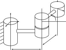
Example 2.2. Twist coordinates for rotation about a line
Consider the rigid displacement generated by rotating about a fixed axis in space, as shown in Figure 2.6. The configuration of the B frame is
given by |
sin α |
cos α |
0 |
l1 |
+ l2 cos α . |
||
gab = |
|||||||
|
|
cos α |
− sin α |
0 |
−l2 sin α |
|
|
|
0 |
0 |
0 |
|
1 |
||
|
|
|
|
|
|
|
|
|
|
0 |
0 |
1 |
|
0 |
|
|
|
|
|
||||
43
B 

z |
|
|
α |
A |
y |
|
x
l2
l1
Figure 2.6: Rigid body displacement generated by rotation about a fixed axis.
We wish to calculate the twist coordinates corresponding to the configuration of the frame B relative to frame A.
To compute the twist which generates gab, we follow the proof of Proposition 2.9, assuming α 6= 0 (so that R 6= I). The axis ω R3 and angle θ R which satisfy exp(ωθb ) = Rab are
0
ω = 0 θ = α,
1
since we are rotating about the z-axis. To find v, we must solve
h I − ec |
ω + ωω |
T |
θi v = pab. |
ωθ |
b |
|
|
|
|
|
Using the fact that θ = α and expanding the left-hand side, this equation becomes
1 |
cos α |
sin α |
0 |
v = |
l1 |
+ l2 cos α . |
||
sin α |
cos α |
− 1 |
0 |
|
−l2 sin α |
|
||
− |
0 |
0 |
|
α |
|
0 |
||
The solution is given by
2 |
sin α |
|
1 |
|
2(1−cos α |
) |
2 |
||
1 |
|
sin α |
||
v = 4 |
−2 |
|
|
|
|
|
2(1−cos α) |
||
|
0 |
|
0 |
|
0 3 2 |
|
−l2 sin α |
3 |
2 |
l1 2 l2 |
3 |
|
||||
|
5 4 |
|
|
|
|
|
5 |
4 |
− |
5 |
|
α |
|
|
|
0 |
|
0 |
|
||||
0 |
|
l |
1 |
+ l |
2 |
cos α |
|
= 6 |
(l1+l2) sin α |
7 |
. |
1 |
|
|
|
|
|
2(1−cos α) |
|
||||
Thus, the twist coordinates for gab are
ξ = |
2(1−0 |
|
|
θ = α = 0. |
||
|
|
l1 |
−l2 |
|
|
|
|
|
|
2 |
|
|
|
|
|
(l1+l2) sin α |
|
|
||
|
|
1 |
α) |
|
||
|
|
|
cos |
|
6 |
|
|
|
0 |
|
|||
|
|
0 |
|
|
||
|
|
|
|
|
|
|
44
p |
ω |
|
θ |
v |
d |
p + θv |
q |
|
|
θ |
|
p |
(a) general screw |
(b) pure translation |
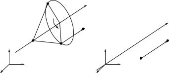
Figure 2.7: Screw motions. |
|
This solution may be unexpected, considering that the motion was generated by a pure rotation about an axis. The reason for the complicated form of the solution is that we took the exponential coordinates of the absolute transformation between the B and A coordinate frames. Consider, instead, the exponential coordinates for the relative transfor-
mation
g(α) = gab(α)gab−1(0),
where gab(0) is the transformation corresponding to α = 0 (a pure translation). It can be verified that the exponential coordinates for the relative transformation g(α) are
l1
0
ξ = 0 θ = α 6= 0.
0
0
1
3.3Screws: a geometric description of twists
In this section, we explore some of the geometric attributes associated with a twist ξ = (v, ω). These attributes give additional insight into the use of twists to parameterize rigid body motions. We begin by defining a specific class of rigid body motions, called screw motions, and then show that a twist is naturally associated with a screw.
Consider a rigid body motion which consists of rotation about an axis in space through an angle of θ radians, followed by translation along the same axis by an amount d as shown in Figure 2.7a. We call such a motion a screw motion, since it is reminiscent of the motion of a screw, in so far as a screw rotates and translates about the same axis. To further encourage this analogy, we define the pitch of the screw to be the ratio of translation to rotation, h := d/θ (assuming θ 6= 0). Thus, the net translational motion after rotating by θ radians is hθ. We represent the
45
p |
ω |
|
|
p − q θ |
ωθ |
|
q + eb (p − q) + hθω |
q |
q + eωθb (p − q)
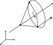
Figure 2.8: Generalized screw motion (with nonzero rotation).
axis as a directed line through a point; choosing q R3 to be a point on the axis and ω R3 to be a unit vector specifying the direction, the axis is the set of points
l = {q + λω : λ R}. |
(2.39) |
The above definitions hold when the screw motion consists of a nonzero rotation followed by translation.
In the case of zero rotation, the axis of the screw must be defined differently: we take the axis as the line through the origin in the direction v (i.e., v is a vector of magnitude 1), as shown in Figure 2.7b. By convention, the pitch of this screw is ∞ and the magnitude is the amount of translation along the direction v. Collecting these, we have the following definition of a screw:
Definition 2.2. Screw motion
A screw S consists of an axis l, a pitch h, and a magnitude M . A screw motion represents rotation by an amount θ = M about the axis l followed by translation by an amount hθ parallel to the axis l. If h = ∞ then the corresponding screw motion consists of a pure translation along the axis of the screw by a distance M .
To compute the rigid body transformation associated with a screw, we analyze the motion of a point p R3, as shown in Figure 2.8. The final location of the point is given by
gp = q + eωθb (p − q) + hθω
or, in homogeneous coordinates,
g |
1 |
= |
e0b |
(I − eb 1 |
1 . |
|
p |
|
ωθ |
ωθ )q + hθω |
p |
46

Since this relationship must hold for all p R3, the rigid motion given
by the screw is |
e0b |
(I − eb 1 |
. |
(2.40) |
g = |
||||
|
ωθ |
ωθ )q + hθω |
|
|
As in the last section, this transformation maps points attached to the rigid body from their initial coordinates (θ = 0) to their final coordinates, and all points are specified with respect to the fixed reference frame.
Note that the rigid body displacement given in equation (2.40) has the same form as the exponential of a twist, given in equation (2.36):
b |
|
0b |
− |
b |
1 |
|
eξθ = |
|
eωθ (I |
|
eωθ )(ω × v) + ωωT vθ . |
||
In fact, if we choose v = −ω × q + hω, then ξ = (v, ω) generates the screw motion in equation (2.40) (assuming kωk = 1, θ 6= 0). In the case of a pure rotation, h = 0 and the twist associated with a screw motion is simply ξ = (−ω × q, ω). In the instance that the screw corresponds to pure translation, we let θ be the amount of translation, and the rigid body motion described by this “screw” is
g = |
I |
θv |
, |
(2.41) |
0 |
1 |
b
which is precisely the motion generated by exp(ξθ) with ξ = (v, 0). Thus, we see that a screw motion corresponds to motion along a constant twist by an amount equal to the magnitude of the screw.
In fact, we can go one step further and define a screw associated
b
with every twist. Let ξ se(3) be a twist with twist coordinates ξ = (v, ω) R6. We do not assume that kωk = 1, allowing both translation plus rotation as well as pure translation. The following are the screw coordinates of a twist:
1. Pitch:
|
ωT v |
|
|
h = |
|
. |
(2.42) |
2 |
|||
|
kωk |
|
|
The pitch of a twist is the ratio of translational motion to rotational motion. If ω = 0, we say that ξ has infinite pitch.
2. Axis: |
( 0 + λv : λ R , |
|
if ω = 0. |
|
|||
|
|
ω×v2 |
+ λω : λ |
|
R |
, if ω = 0 |
(2.43) |
|
l = {kωk |
|
} |
6 |
|||
|
{ |
|
} |
|
|
|
|
The axis l is a directed line through a point. For ω 6= 0, the axis is
a line in the ω direction going through the point ω×v . For ω = 0,
kωk2
the axis is a line in the v direction going through the origin.
47

3. Magnitude: |
( |
|
|
|
|
|
|
M = |
kωk, |
if ω 6= 0 |
(2.44) |
|
kvk, |
if ω = 0. |
|
The magnitude of a screw is the net rotation if the motion contains
a rotational component, or the net translation otherwise. If we
k k k k b choose ω = 1 (or v = 1 when ω = 0), then a twist ξθ has
magnitude M = θ.
We next show that given a screw, we can define a twist which realizes the screw motion and has the proper geometric attributes. It su ces to prove that we can define a twist with a given set of attributes, since any twist with those attributes will generate the correct screw motion.
Proposition 2.10. Screw motions correspond to twists
Given a screw with axis l, pitch h, and magnitude M , there exists a unit magnitude twist ξ such that the rigid motion associated with the screw is generated by the twist M ξ.
Proof. The proof is by construction. We split the proof into the usual cases: pure translation and translation plus rotation. For consistency, we
b
generate a screw of the form ξθ, where θ = M . We will assume that q is a point on the axis of the screw.
Case 1 (h = ∞). Let l = {q + λv : kvk = 1, λ R}, θ = M , and define
ξ = |
0 |
v . |
b |
0 |
0 |
b
The rigid body motion exp(ξθ) corresponds to pure translation along the screw axis by an amount θ.
Case 2 (h finite). Let l = {q + λω : kωk = 1, λ R}, θ = M , and define
ξ = |
|
0 |
− |
ω |
× |
0 |
. |
b |
|
ω |
|
|
q + hω |
|
|
|
b |
|
|
|
|
|
b
The fact that the rigid body motion exp(ξθ) is the appropriate screw motion is verified by direct calculation. 

There are several important special cases of screw motion of which we shall make frequent use. A zero pitch screw is a screw motion for which h = 0, corresponding to a pure rotation about an axis. Zero pitch screws are used to model the action of a revolute joint of a manipulator. The axis of the screw corresponds to the axis of rotation of the joint. An infinite pitch screw is a motion for which h = ∞, as previously mentioned. This case corresponds to a pure translation and is the model for the action of a prismatic joint. The axis of the screw is defined to be a line through
48
the origin which points in the direction of translation (a line through any other point could also be used). The magnitude of the screw gives the amount of the displacement. Finally, we define a unit twist to be a twist such that either kωk = 1, or ω = 0 and kvk = 1; that is, a unit twist has magnitude M = 1. Unit twists are useful since they allow us to express
b
rigid motions due to revolute and prismatic joints as g = exp(ξθ), where θ corresponds to the amount of rotation or translation.
Some comments about the point q on the axis of the screw in the formulas above are in order. For instance, it is important to note that the formulas do not change for di erent choices of points on the axis of the screw. Thus, if q′ = q + λω is some other point on the axis of the screw, the formula in equation (2.40) would be unchanged. It is also instructive to verify that for points on the axis of the screw, the screw motion is purely translational of magnitude hθ, as may be verified by applying equation (2.40) to points on the axis.
The geometric meaning of a screw is expressed succinctly in the following theorem. Its proof follows directly from the definition of the attributes of a twist.
Theorem 2.11 (Chasles). Every rigid body motion can be realized by a rotation about an axis combined with a translation parallel to that axis.
As mentioned previously, it is important to keep in mind that the
exponential of a twist represents the relative motion of a rigid body. As a
b 3 mapping, exp(ξθ) takes points from their initial coordinates, p(0) R ,
to their coordinates after the rigid motion is applied:
b
p(θ) = eξθ p(0).
Both p(0) and p(θ) are specified with respect to a single reference frame. If a coordinate frame B is attached to a rigid body undergoing a screw motion, the instantaneous configuration of the coordinate frame B, relative to a fixed frame A, is given by
ξθ |
(2.45) |
gab(θ) = eb gab(0). |
This transformation can be interpreted as follows: multiplication by gab(0) maps the coordinates of a point relative to the B frame into A’s coordinates, and the exponential map transforms the point to its final location (still in A coordinates).
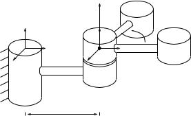
Example 2.3. Rotation about a line
Consider the motion of a rigid body rotating about a fixed axis in space, as shown in Figure 2.9. This motion corresponds to a zero-pitch screw about an axis in the ω = (0, 0, 1) direction passing through the point
49
|
|
ω |
z |
|
θ |
|
|
|
A |
|
B |
y |
q |
|
x |
|
|
|
|
l1
Figure 2.9: Rigid body motion generated by rotation about a fixed axis.
q = (0, l1, 0). The corresponding twist is |
|
|
|
|
|
|
|||||||||
|
|
|
ξ = |
− |
ω× |
|
= |
0 |
. |
|
|
|
|
||
|
|
|
|
|
|
|
|
|
|
0 |
|
|
|
|
|
|
|
|
|
|
ω |
|
q |
l1 |
|
|
|
|
|||
|
|
|
|
|
|
0 |
|
|
|
|
|
||||
|
|
|
|
|
|
|
|
|
|
1 |
|
|
|
|
|
|
|
|
|
|
|
|
|
|
|
0 |
|
|
|
|
|
The exponential of this twist is given by |
|
|
|
|
(1 cos θ) . |
||||||||||
eξθ = |
eωθ |
(I eωθ )(ω |
|
v) |
= |
sin θ |
|
cos θ |
0 |
l1 |
|||||
|
0b |
− b 1 |
|
|
|
|
|
cos θ |
− sin θ |
0 |
|
l1 sin θ |
|
||
b |
|
× |
|
0 |
|
0 |
1 |
|
−0 |
||||||
|
|
|
|
|
|
|
0 |
|
0 |
0 |
|
1 |
|||
|
|
|
|
|
|
|
|
|
|
|
|
|
|
|
|
|
|
|
|
|
|
|
|
|
|
|
|
|
|
|
|
When applied to the homogeneous representation of a point, this matrix maps the coordinates of a point on the rigid body, specified relative to the frame A with θ = 0, to the coordinates of the same point after rotating by θ radians about the axis.
The rigid transformation which maps points in B coordinates to A coordinates—and hence describes the configuration of the rigid body—is
b
given by gab(θ) = exp(ξθ)gab(0) where
gab(0) = "0 |
h |
1 i# . |
I |
|
0 |
|
l1 |
|
|
|
0 |
Taking the exponential and performing the matrix multiplication yields
gab = |
sin θ |
cos θ |
0 |
l1 |
, |
|
|
|
cos θ |
− sin θ |
0 |
0 |
|
|
0 |
0 |
1 |
0 |
||
|
|
|
|
|
|
|
|
|
|
|
|
|
|
00 0 1
which can be verified by inspection.
50

4Velocity of a Rigid Body
In this section, we derive a formula for the velocity of a rigid body whose motion is given by g(t), a curve parameterized by time t in SE(3). This is not such a naive question as in the case of a single particle following
a curve q(t) R3, where the velocity of the particle is vq (t) = dtd q(t), because this notion of velocity cannot be generalized since SE(3) is not
Euclidean. In particular, the quantity g˙(t) / SE(3) and g˙(t) / se(3) and the question of its connection with rotational and translational velocity needs to be handled with care. Further, the definition of velocity needs to relate to our informal understanding of rotational and translational velocity. We will show that the proper representation of rigid body velocity is through the use of twists.
4.1Rotational velocity
Consider first the case of pure rotational motion in R3. Let Rab(t) SO(3) be a curve representing a trajectory of an object frame B, with origin at the origin of frame A, but rotating relative to the fixed frame A. We call A the spatial coordinate frame and B the body coordinate frame.1 Any point q attached to the rigid body follows a path in spatial coordinates given by
qa(t) = Rab(t)qb.
Note that the coordinates qb are fixed in the body frame. The velocity of the point in spatial coordinates is
|
|
d |
˙ |
|
vqa |
(t) = |
dt |
qa(t) = Rab(t)qb. |
(2.46) |
|
|
|
|
˙
Thus Rab maps the body coordinates of a point to the spatial velocity of that point. This representation of the rotational velocity is somewhat ine cient, since it requires nine numbers to describe the velocity of a
˙
rotating body. One may use the special structure in the matrix Rab to derive a more compact representation. To this end, we rewrite equation (2.46) as
vqa (t) = R˙ ab(t)Rab−1(t)Rab(t)qb. |
(2.47) |
||
˙ |
−1 |
(t) so(3); i.e., it is skew- |
|
The following lemma shows that Rab(t)Rab |
|||
symmetric.
˙ −1 3×3
Lemma 2.12. Given R(t) SO(3), the matrices R(t)R (t) R
˙
and R−1(t)R(t) R3×3 are skew-symmetric.
1The word “spatial” is sometimes used to di erentiate between planar motions in R2 and general (spatial) motions in R3. In this chapter we reserve the word spatial to mean “relative to a fixed (inertial) coordinate frame.”
51

Proof. Di erentiating the identity
R(t)R(t)T = I
we have, dropping the dependence of the matrices on t,
˙ |
|
T |
˙ T |
= 0, |
||
RR |
|
+ RR |
||||
so that |
|
|
|
|
|
|
˙ |
T |
˙ |
T |
T |
. |
|
RR |
|
|
= −(RR ) |
|
||
˙ −1 ˙ T −1 ˙ Hence, RR = RR is a skew-symmetric matrix. The proof that R R
is skew-symmetric follows by di erentiating the identity RT R = I.
Lemma 2.12 allows us to represent the velocity of a rotating body using a 3-vector. We define the instantaneous spatial angular velocity, denoted ωabs R3, as
s |
˙ |
−1 |
(2.48) |
ωbab := RabRab . |
|||
The vector ωabs corresponds to the instantaneous angular velocity of the object as seen from the spatial (A) coordinate frame. Similarly, we define the instantaneous body angular velocity, denoted ωabb R3, as
b |
−1 ˙ |
(2.49) |
ωbab := Rab Rab. |
||
The body angular velocity describes the angular velocity as viewed from the instantaneous body (B) coordinate frame. From these two equations, it follows that the relationship between the two angular velocities is
ωbabb = Rab−1ωbabs Rab or ωabb = Rab−1ωabs . |
(2.50) |
Thus the body angular velocity can be determined from the spatial angular velocity by rotating the angular velocity vector into the instantaneous body frame.
Returning now to equation (2.47), we can express the velocity of a point in terms of the instantaneous angular velocity of the rigid body. Substituting equation (2.48) into equation (2.47),
vqa (t) = ωbabs Rab(t)qb = ωabs (t) × qa(t). |
(2.51) |
Alternatively, using equation (2.50), the velocity of the point in body frame is given by
vqb (t) := RabT (t)vqa (t) = ωabb (t) × qb. |
(2.52) |
Equations (2.51) and (2.52) constitute a compact description of the velocity of all particles of the body in terms of the body and spatial angular velocities, ωabb and ωabs .
52