mls94-complete[1]

not having a singularity at the identity orientation, R = I, though they do contain singularities at other, di erent, orientations. For example, in the instance of ZYX Euler angles, we have:

Rab = Rz(ψ)Ry(θ)Rx(φ) = ebzψ eybθ exbφ,

which is singular when θ = −π/2. It is a fundamental topological fact that singularities can never be eliminated in any 3-dimensional representation of SO(3). This situation is similar to that of attempting to find a global coordinate chart on a sphere, which also fails.

Quaternions

Quaternions generalize complex numbers and can be used to represent rotations in much the same way as complex numbers on the unit circle can be used to represent planar rotations. Unlike Euler angles, quaternions give a global parameterization of SO(3), at the cost of using four numbers instead of three to represent a rotation.

Formally, a quaternion is a vector quantity of the form

Q = q0 + q1i + q2j + q3k qi R, i = 0, . . . , 3,

where q0 is the scalar component of Q and ~q = (q1, q2, q3) is the vector component. A convenient shorthand notation is Q = (q0, ~q ) with q0 R, ~q R3. The set of quaternions Q is a 4-dimensional vector space over the reals and forms a group with respect to quaternion multiplication, denoted “·”. Multiplication is distributive and associative, but not commutative; it satisfies the relations

The conjugate of a quaternion Q = (q0, ~q ) is given by Q = (q0, −~q ) and the magnitude of a quaternion satisfies

kQk2 = Q · Q = q02 + q12 + q22 + q32.

It is straightforward to verify that the inverse of a quaternion is Q−1 = Q /kQk2 and that Q = (1, 0) is the identity element for quaternion multiplication.

The product between two quaternions has a simple form in terms of the inner and cross products between vectors in R3. Let Q = (q0, ~q ) and P = (p0, p~ ) be quaternions, where q0, p0 R are the scalar parts of Q and P and ~q, p~ are the vector parts. It can be shown algebraically that the product of two quaternions satisfies:

Q · P = (q0p0 − ~q · p,~ q0p~ + p0~q + ~q × p~ ).

33

In most applications, this formula eliminates the need to make direct use of the multiplicative relations given above.

The unit quaternions are the subset of all Q Q such that kQk = 1. The unit quaternions also form a group with respect to quaternion multiplication (Exercise 6). Given a rotation matrix R = exp(ωθb ), we define the associated unit quaternion as

Q = cos(θ/2), ω sin(θ/2) ,

where ω R3 represents the unit axis of rotation and θ R represents the angle of rotation. A detailed calculation shows that if Qab represents a rotation between frame A and frame B, and Qbc represents a rotation between frames B and C, then the rotation between A and C is given by the quaternion

Qac = Qab · Qbc.

Thus, the group operation on unit quaternions directly corresponds to the group operation for rotations. Given a unit quaternion Q = (q0, ~q ), we can extract the corresponding rotation by setting

and R = exp(ωθb ).

Since the group structure for quaternions directly corresponds to that of rotations, quaternions provide an e cient representation for rotations which do not su er from singularities. Their properties are explored more fully in the exercises.

3Rigid Motion in R3

Recall from Section 1 that a rigid motion is one that preserves the distance between points and the angle between vectors. We represent rigid motions by using rigid body transformations to describe the instantaneous position and orientation of a body coordinate frame relative to an inertial frame. This representation relies on the fact that rigid body transformations map right-handed, orthonormal frames to right-handed, orthonormal frames, thus preserving distance and angles. In this book we refer to all transformations between coordinate frames as rigid body transformations (or just rigid transformations), whether or not a rigid body is explicitly present.

In general, rigid motions consist of rotation and translation. In the preceding section, we discussed representations of pure rotational motion. The procedure for representing pure translational motion is very simple: choose a (any) point in the body and keep track of the coordinates of the

34

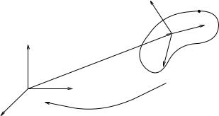
Figure 2.3: Coordinate frames for specifying rigid motions.

point relative to some known frame. This gives a curve p(t) R3, t [0, T ], for a trajectory of the entire rigid body.

The representation of general rigid body motion, involving both translation and rotation, is more involved. We describe the position and orientation of a coordinate frame B attached to the body relative to an inertial frame A (see Figure 2.3). Let pab R3 be the position vector of the origin of frame B from the origin of frame A, and Rab SO(3) the orientation of frame B, relative to frame A. A configuration of the system consists of the pair (pab, Rab), and the configuration space of the system is the product space of R3 with SO(3), which shall be denoted as

We defer the proof of the fact that SE(3) is a group to the next subsection. As in the case of SO(3), there is a generalization to n dimensions,

SE(n) := Rn × SO(n).

Analogous to the rotational case, an element (p, R) SE(3) serves as both a specification of the configuration of a rigid body and a transformation taking the coordinates of a point from one frame to another. More precisely, let qa, qb R3 be the coordinates of a point q relative to frames A and B, respectively. Given qb, we can find qa by a transformation of coordinates:

where gab = (pab, Rab) SE(3) is the specification of the configuration of the B frame relative to the A frame. By an abuse of notation, we write g(q) to denote the action of a rigid transformation on a point,

g(q) = p + Rq,

35

so that qa = gab(qb).

The action of a rigid transformation g = (p, R) on a vector v = s − r is defined by the following formula:

g (v) := g(s) − g(r) = R(s − r) = Rv.

Thus, a vector is transformed by rotation.

3.1Homogeneous representation

The transformation of points and vectors by rigid transformations has a simple representation in terms of matrices and vectors in R4. We begin by adopting some notation. We append 1 to the coordinates of a point

These are called the homogeneous coordinates of the point q. Thus, the origin has the form

¯

O =

Vectors, which are the di erence of points, then have the form

Note that the form of the vector is di erent from that of a point. The 0 and 1 in the fourth component of vectors and points, respectively, will remind us of the di erence between points and vectors and enforce a few rules of syntax:

1.Sums and di erences of vectors are vectors.

2.The sum of a vector and a point is a point.

3.The di erence between two points is a vector.

4.The sum of two points is meaningless.

The transformation qa = gab(qb) given in equation (2.22) is an a ne transformation. Using the preceding notation for points, we may repre-

The 4 × 4 matrix g¯ab is called the homogeneous representation of gab SE(3). In general, if g = (p, R) SE(3), then

36

The price to be paid for the convenience of having a homogeneous or linear representation of the rigid body motion is the increase in the dimension of the quantities involved from 3 to 4.

The last row of the matrix of equation (2.23) appears to be “extra baggage” as well. However, in the graphics literature, the number 1 is frequently replaced by a scalar constant which is either greater than 1 to represent dilation or less than 1 to represent contraction. Also, the row vector of zeros in the last row may be replaced by some other row vector to provide “perspective transformations.” In both these instances, of course, the transformation represented by the augmented matrix no longer corresponds to a rigid displacement.

Rigid body transformations can be composed to form new rigid body transformations. Let gbc SE(3) be the configuration of a frame C relative to a frame B, and gab the configuration of frame B relative to another frame A. Then, using equation (2.23), the configuration of C relative to frame A is given by

Equation (2.24) defines the composition rule for rigid body transformations to be the standard matrix multiplication. Using the homogeneous representation, it may be verified that the set of rigid transformations is a group; that is:

1.If g1, g2 SE(3), then g1g2 SE(3).

2.The 4 × 4 identity element, I, is in SE(3).

3.If g SE(3), then the inverse of g¯ is determined by straightforward matrix inversion to be:

so that g−1 = (−RT p, RT ).

4. The composition rule for rigid body transformations is associative.

Using the homogeneous representation for a vector v = s−r, we obtain the representation for a rigid body transformation of v by multiplying the homogeneous representations of v by the homogeneous representation of

Note that by defining the homogeneous representation of a vector to have a zero in the bottom row, we are able to once again use matrix multiplication to represent the action of a rigid transformation, this time on

37

the amount of rotation, then the orientation of coordinate frame B with

The coordinates for the origin of frame B are

0 pab = l1 ,

0

again relative to frame A. The homogeneous representation of the con-

Note that when the angle θ = 0, gab(0) gives that the relative displacement between the two frames is a pure translation along the y-axis.

3.2Exponential coordinates for rigid motion and twists

The notion of the exponential mapping introduced in Section 2 for SO(3) can be generalized to the Euclidean group, SE(3). We will make extensive use of this representation in the sequel since it allows an elegant, rigorous, and geometric treatment of spatial rigid body motion. We begin by presenting a pair of motivational examples and then present a formal set of definitions.

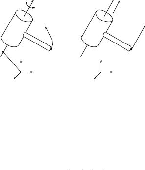
Consider the simple example of a one-link robot as shown in Figure 2.5a, where the axis of rotation is ω R3, kωk = 1, and q R3 is a point on the axis. Assuming that the link rotates with unit velocity, then the velocity of the tip point, p(t), is

This equation can be conveniently converted into homogeneous coordi-

× b nates by defining the 4 4 matrix ξ to be

39

An element of se(3) is referred to as a twist, or a (infinitesimal) generator of the Euclidean group. We define the (vee) operator to extract the

Proof. The proof is by explicit calculation. In the course of the proof, we

Case 1 (ω = 0). If ω = 0, then a straightforward calculation shows that

which is in SE(3) as desired.

Case 2 (ω 6= 0). Assume kωk = 1, by appropriate scaling of θ if necessary, and define a rigid transformation g by

Now, using the calculation of Lemma 2.3, with kωk = 1, we have

41

where h := ωT v. Using the following identity (see Exercise 8),

b′

it su ces to calculate exp(ξ θ). This simplifies the calculation since it may be verified (using ωωb = ω × ω = 0) that

which is an element of SE(3).

b

The transformation g = exp(ξθ) is slightly di erent than the rigid transformations that we have encountered previously. We interpret it not as mapping points from one coordinate frame to another, but rather as mapping points from their initial coordinates, p(0) R3, to their coordinates after the rigid motion is applied:

b

p(θ) = eξθ p(0).

In this equation, both p(0) and p(θ) are specified with respect to a single reference frame. Similarly, if we let gab(0) represent the initial configuration of a rigid body relative to a frame A, then the final configuration, still with respect to A, is given by

Thus, the exponential map for a twist gives the relative motion of a rigid body. This interpretation of the exponential of a twist as a mapping from initial to final configurations will be especially important as we study the kinematics of robot mechanisms in the next chapter.

Our primary interest is to use the exponential map as a representation for rigid motion, and hence we must show that every rigid transformation can be written as the exponential of some twist. The following proposition asserts that this is always possible and gives a constructive procedure for finding the twist which generates a given rigid transformation.

Proposition 2.9. Surjectivity of the exponential map onto SE(3)

42