mls94-complete[1]

(d)Find the spatial Jacobian of the structure equations. Give an explicit answer. Use the fact that some links intersect at a point to minimize extra calculations.

(e)Find the singular configurations of the mechanism. In addition to kinematic singularities, also identify any actuator singularities.

22.Stewart platform

Consider the Stewart platform shown in Figure 3.21. Let θi represent the displacement of the ith prismatic actuator.

(a)Use Gruebler’s formula to compute the number of degrees of freedom of the mechanism.

(b)Show that if θi > 0 for all i, then the mechanism is not at a singular configuration.

(c)Suppose that we replace the spherical joints in the Stewart platform with U-joints (a U-joint consists of two orthogonal revolute joints which intersect at a point). Use Gruebler’s formula to compute the number of degrees of freedom of the mechanism.

(d)Derive the structure equations for the mechanism in part (c). Are there any singular configurations?

153

Chapter 4

Robot Dynamics and

Control

This chapter presents an introduction to the dynamics and control of robot manipulators. We derive the equations of motion for a general open-chain manipulator and, using the structure present in the dynamics, construct control laws for asymptotic tracking of a desired trajectory. In deriving the dynamics, we will make explicit use of twists for representing the kinematics of the manipulator and explore the role that the kinematics play in the equations of motion. We assume some familiarity with dynamics and control of physical systems.

1Introduction

The kinematic models of robots that we saw in the last chapter describe how the motion of the joints of a robot is related to the motion of the rigid bodies that make up the robot. We implicitly assumed that we could command arbitrary joint level trajectories and that these trajectories would be faithfully executed by the real-world robot. In this chapter, we look more closely at how to execute a given joint trajectory on a robot manipulator.

Most robot manipulators are driven by electric, hydraulic, or pneumatic actuators, which apply torques (or forces, in the case of linear actuators) at the joints of the robot. The dynamics of a robot manipulator describes how the robot moves in response to these actuator forces. For simplicity, we will assume that the actuators do not have dynamics of their own and, hence, we can command arbitrary torques at the joints of the robot. This allows us to study the inherent mechanics of robot manipulators without worrying about the details of how the joints are actuated on a particular robot.

155

We will describe the dynamics of a robot manipulator using a set of nonlinear, second-order, ordinary di erential equations which depend on the kinematic and inertial properties of the robot. Although in principle these equations can be derived by summing all of the forces acting on the coupled rigid bodies which form the robot, we shall rely instead on a Lagrangian derivation of the dynamics. This technique has the advantage of requiring only the kinetic and potential energies of the system to be computed, and hence tends to be less prone to error than summing together the inertial, Coriolis, centrifugal, actuator, and other forces acting on the robot’s links. It also allows the structural properties of the dynamics to be determined and exploited.

Once the equations of motion for a manipulator are known, the inverse problem can be treated: the control of a robot manipulator entails finding actuator forces which cause the manipulator to move along a given trajectory. If we have a perfect model of the dynamics of the manipulator, we can find the proper joint torques directly from this model. In practice, we must design a feedback control law which updates the applied forces in response to deviations from the desired trajectory. Care is required in designing a feedback control law to insure that the overall system converges to the desired trajectory in the presence of initial condition errors, sensor noise, and modeling errors.

In this chapter, we primarily concentrate on one of the simplest robot control problems, that of regulating the position of the robot. There are two basic ways that this problem can be solved. The first, referred to as joint space control, involves converting a given task into a desired path for the joints of the robot. A control law is then used to determine joint torques which cause the manipulator to follow the given trajectory. A di erent approach is to transform the dynamics and control problem into the task space, so that the control law is written in terms of the end- e ector position and orientation. We refer to this approach as workspace control.

A much harder control problem is one in which the robot is in contact with its environment. In this case, we must regulate not only the position of the end-e ector but also the forces it applies against the environment. We discuss this problem briefly in the last section of this chapter and defer a more complete treatment until Chapter 6, after we have introduced the tools necessary to study constrained systems.

2Lagrange’s Equations

There are many methods for generating the dynamic equations of a mechanical system. All methods generate equivalent sets of equations, but di erent forms of the equations may be better suited for computation or analysis. We will use a Lagrangian analysis for our derivation, which

156

relies on the energy properties of mechanical systems to compute the equations of motion. The resulting equations can be computed in closed form, allowing detailed analysis of the properties of the system.

2.1Basic formulation

Consider a system of n particles which obeys Newton’s second law—the time rate of change of a particle’s momentum is equal to the force applied to a particle. If we let Fi be the applied force on the ith particle, mi be the particle’s mass, and ri be its position, then Newton’s law becomes

Our interest is not in a set of independent particles, but rather in particles which are attached to one another and have limited degrees of freedom. To describe this interconnection, we introduce constraints between the positions of our particles. Each constraint is represented by a function gj : R3n → R such that

gj (r1, . . . , rn) = 0 j = 1, . . . , k. (4.2)

A constraint which can be written in this form, as an algebraic relationship between the positions of the particles, is called a holonomic constraint. More general constraints between rigid bodies—involving r˙i—can also occur, as we shall discover when we study multifingered hands.

A constraint acts on a system of particles through application of constraint forces. The constraint forces are determined in such a way that the constraint in equation (4.2) is always satisfied. If we view the constraint as a smooth surface in Rn, the constraint forces are normal to this surface and restrict the velocity of the system to be tangent to the surface at all times. Thus, we can rewrite our system dynamics as a vector equation

where the vectors 1, . . . , k R3n are a basis for the forces of constraint and λj is the scale factor for the jth basis element. We do not require that1, . . . , k be orthonormal. For constraints of the form in equation (4.2),j can be taken as the gradient of gj , which is perpendicular to the level set gj (r) = 0.

The scalars λ1, . . . , λk are called Lagrange multipliers. Formally, we determine the Lagrange multipliers by solving the 3n + k equations in equations (4.2) and (4.3) for the 3n + k variables r R3n and λ Rk. The λi values only give the relative magnitudes of the constraint forces since the vectors j are not necessarily orthonormal.

157

This approach to dealing with constraints is intuitively simple but computationally complex, since we must keep track of the state of all particles in the system even though they are not capable of independent motion. A more appealing approach is to describe the motion of the system in terms of a smaller set of variables that completely describes the configuration of the system. For a system of n particles with k constraints, we seek a set of m = 3n − k variables q1, . . . , qm and smooth functions f1, . . . , fn such that

We call the qi’s a set of generalized coordinates for the system. For a robot manipulator consisting of rigid links, these generalized coordinates are almost always chosen to be the angles of the joints. The specification of these angles uniquely determines the position of all of the particles which make up the robot.

Since the values of the generalized coordinates are su cient to specify the position of the particles, we can rewrite the equations of motion for the system in terms of the generalized coordinates. To do so, we also express the external forces applied to the system in terms of components along the generalized coordinates. We call these forces generalized forces to distinguish them from physical forces, which are always represented as vectors in R3. For a robot manipulator with joint angles acting as generalized coordinates, the generalized forces are the torques applied about the joint axes.

To write the equations of motion, we define the Lagrangian, L, as the di erence between the kinetic and potential energy of the system. Thus,

L(q, q˙) = T (q, q˙) − V (q),

where T is the kinetic energy and V is the potential energy of the system, both written in generalized coordinates.

Theorem 4.1. Lagrange’s equations

The equations of motion for a mechanical system with generalized coordinates q Rm and Lagrangian L are given by

where Υi is the external force acting on the ith generalized coordinate.

The equations in (4.5) are called Lagrange’s equations. We will often write them in vector form as

158

l

θ

φ

mg

Figure 4.1: Idealized spherical pendulum. The configuration of the system is described by the angles θ and φ.

where ∂L∂q˙ , ∂L∂q , and Υ are to be formally regarded as row vectors, though we often write them as column vectors for notational convenience. A proof of Theorem 4.1 can be found in most books on dynamics of mechanical systems (e.g., [99]).

Lagrange’s equations are an elegant formulation of the dynamics of a mechanical system. They reduce the number of equations needed to describe the motion of the system from n, the number of particles in the system, to m, the number of generalized coordinates. Note that if there

are no constraints, then we can choose q to be the components of r, giving

P

T = 12 mikr˙i2k, and equation (4.5) then reduces to equation (4.1). In fact, rearranging equation (4.5) as

is just a restatement of Newton’s law in generalized coordinates:

dtd (momentum) = applied force.

The motion of the individual particles can be recovered through application of equation (4.4).

Example 4.1. Dynamics of a spherical pendulum

Consider an idealized spherical pendulum as shown in Figure 4.1. The system consists of a point with mass m attached to a spherical joint by a massless rod of length l. We parameterize the configuration of the point mass by two scalars, θ and φ, which measure the angular displacement from the z- and x-axes, respectively. We wish to solve for the motion of the mass under the influence of gravity.

159

We begin by deriving the Lagrangian for the system. The position of the mass, relative to the origin at the base of the pendulum, is given by

and the potential energy is

V = −mgl cos θ,

where g ≈ 9.8 m/sec2 is the gravitational constant. Thus, the Lagrangian is given by

(4.7) Given the initial position and velocity of the point mass, equation (4.7) uniquely determines the subsequent motion of the system. The motion of the mass in R3 can be retrieved from equation (4.6).

2.2Inertial properties of rigid bodies

To apply Lagrange’s equations to a robot, we must calculate the kinetic and potential energy of the robot links as a function of the joint angles

160

r

A

g

Figure 4.2: Coordinate frames for calculating the kinetic energy of a moving rigid body.

and velocities. This, in turn, requires that we have a model for the mass distribution of the links. Since each link is a rigid body, its kinetic and potential energy can be defined in terms of its total mass and its moments of inertia about the center of mass.

Let V R3 be the volume occupied by a rigid body, and ρ(r), r V be the mass distribution of the body. If the object is made from a homogeneous material, then ρ(r) = ρ, a constant. The mass of the body is the volume integral of the mass density:

Z

m = ρ(r) dV.

V

The center of mass of the body is the weighted average of the density:

Z

r¯ = 1 ρ(r)r dV. m V

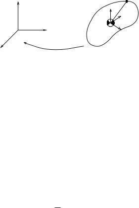
Consider the rigid object shown in Figure 4.2. We compute the kinetic energy as follows: fix the body frame at the mass center of the object and let (p, R) be a trajectory of the object relative to an inertial frame, where we have dropped all subscripts to simplify notation. Let r R3 be the coordinates of a body point relative to the body frame. The velocity of the point in the inertial frame is given by

˙

p˙ + R r

Expanding the product in the kinetic energy integral yields

161

The first term of the above expression gives the translational kinetic energy. The second term vanishes because the body frame is placed at the mass center of the object and

Z Z

T ˙ T ˙

ρ(r)(p˙ R)r dV = (p˙ R) ρ(r)r dV = 0.

V V

The last term can be simplified using properties of rotation and skewsymmetric matrices:

is called the inertia tensor of the object expressed in the body frame. It has entries Z

Ixx = ρ(r)(y2 + z2) dx dy dz

VZ

Ixy = − ρ(r)(xy) dx dy dz,

V

and the other entries are defined similarly.

The total kinetic energy of the object can now be written as the sum of a translational component and a rotational component,

b

generalized inertia matrix of the object, expressed in the body frame. The matrix M is symmetric and positive definite.

Example 4.2. Generalized inertia matrix for a homogeneous bar

Consider a homogeneous rectangular bar with mass m, length l, width w, and height h, as shown in Figure 4.3. The mass density of the bar is

162