mls94-complete[1]

l

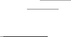
Figure 4.12: Planar manipulator moving in a slot.

6.3Example: A planar manipulator moving in a slot

As a simple example of a constrained manipulator, consider the control of a two degree of freedom, planar manipulator whose end-e ector is forced to lie in a slot, as shown in Figure 4.12. This system resembles a slidercrank mechanism, except that we are allowed to apply torques on both revolute joints, allowing us to control both the motion of the slider as well as the force applied against the slot. This example is easily adapted to a robot pushing against a wall, in which case the forces against the slot must always be pointed in a preferred direction.

We take the slot to be a straight line passing through the point q = (l, 0) and making an angle α with respect to the x-axis of the base frame. The vector normal to the direction of the slot is given by

and the slot can be described as the set of all points p R2 such that (p − q) · n = 0.

The constraint on the manipulator is obtained by requiring that the position of the end-e ector remain in the slot. Letting p(θ) R2 represent the position of the tool frame, this constraint becomes

Substituting the forward kinematics of the manipulator yields

h(θ) = (l1 cos θ1 + l2 cos(θ1 + θ2) − l) sin α

−(l1 sin θ1 + l2 sin(θ1 + θ2)) cos α

=−l1 sin(θ1 − α) − l2 sin(θ1 + θ2 − α) − l sin α.

203

The gradient of the constraint, which gives the direction of the normal force, is given by

Note that this is the direction of the normal force in joint coordinates. That is, joint torques applied in this direction will cause no motion, only forces against the side of the slot.

To parameterize the allowable motion along the slot, we let s R represent the position along the slot, with s = 0 denoting the point q = (l, 0). Finding a function f (s) such that h(f (s)) = 0 involves solving the inverse kinematics of the manipulator: given the position along the slot, we must find joint angles which achieve that position.

If the end of the manipulator is at a position s along the slot, then the xy coordinates of the end-e ector are

x(s) = l + s cos α y(s) = s sin α.

Solving the inverse kinematics (see Chapter 3, Section 3) and assuming the elbow down solution, we have

√2(s+l cos α)

4l12l22−(s2+2ls cos α+l2−l12−l22)2

(after some simplification).

This matrix can now be used to compute the equations of motion and derive an appropriate control law. In particular, the computed torque

controller has the form

− − ˙ ˙

τ = M (θ)J (¨sd Kv e˙s Kpes) + C(θ, θ)J + M (θ)J s˙ + λn,

where es = s − sd; λ is the desired force against the slot; Kv , Kp R are the gain and damping factors; and M and C are the generalized inertial and Coriolis matrices. The inertial parameters were calculated in

204

where

α = Iz1 + Iz2 + m1r12 + m2(l12 + r22)

β= m2l1l2

δ= Iz2 + m2r22.

It is perhaps surprising that such a simple problem can have such an unwieldy solution. The di culty is that we have cast the entire problem into the joint space of the manipulator, where the constraint θ = f (s) is a very complex looking curve.

A better way of deriving the equations of motion for this system is to rewrite the dynamics of the system in terms of workspace variables which describe the position of the end-e ector (see Exercise 12). Once written in this way, the constraint that the end of the manipulator remain in the slot is a very simple one. This is the basic approach used in Chapter 6, where we present a general framework which incorporates this example and many other constrained manipulation systems.

205

7Summary

The following are the key concepts covered in this chapter:

1.The equations of motion for a mechanical system with Lagrangian

L = T (q, q˙) − V (q) satisfies Lagrange’s equations:

where q Rn is a set of generalized coordinates for the system and

Υ Rn represents the vector of generalized external forces.

2.The equations of motion for a rigid body with configuration g(t)

SE(3) are given by the Newton-Euler equations:

and applied body wrench.

3.The equations of motion for an open-chain robot manipulator can be written as

¨ ˙ ˙ ˙

M (θ)θ + C(θ, θ)θ + N (θ, θ) = τ

where θ Rn is the set of joint variables for the robot and τ Rn is the set of actuator forces applied at the joints. The dynamics of a robot manipulator satisfy the following properties:

(a) M (θ) is symmetric and positive definite.

˙ − n×n

(b) M 2C R is a skew-symmetric matrix.

4. An equilibrium point x for the system x˙ = f (x, t) is locally asymptotically stable if all solutions which start near x approach x as t → ∞. Stability can be checked using the direct method of Lyapunov, by finding a locally positive definite function V (x, t) ≥ 0

− ˙

such that V (x, t) is a locally positive definite function along tra-

− ˙

jectories of the system. In situations in which V is only positive semi-definite, Lasalle’s invariance principle can be used to check asymptotic stability. Alternatively, the indirect method of Lyapunov can be employed by examining the linearization of the system, if it exists. Global exponential stability of the linearization implies local exponential stability of the full nonlinear system.

206

5.Using the form and structure of the robot dynamics, several control laws can be shown to track arbitrary trajectories. Two of the most common are the computed torque control law,

¨ ˙ ˙ ˙

τ = M (θ)(θd + Kv e˙ + Kpe) + C(θ, θ)θ + N (θ, θ),

and an augmented PD control law,

¨ ˙ ˙ ˙

τ = M (θ)θd + C(θ, θ)θd + N (θ, θ) + Kv e˙ + Kpe.

Both of these controllers result in exponential trajectory tracking of a given joint space trajectory. Workspace versions of these control laws can also be derived, allowing end-e ector trajectories to be tracked without solving the inverse kinematics problem. Stability of these controllers can be verified using Lyapunov stability.

8Bibliography

The Lagrangian formulation of dynamics is classical; a good treatment can be found in Rosenberg [99] or Pars [89]. Its application to the dynamics of a robot manipulator can be found in most standard textbooks on robotics, for example [2, 21, 35, 52, 110].

The geometric formulation of the equations of motion for kinematic chains presented in Section 3.3 is based on the recent work of Brockett, Stokes, and Park [15, 87]. This is closely related to the spatial operator algebra formulation of Rodriguez, Jain, and Kreutz-Delgado [45, 98], in which the tree-like nature of the system is more fully exploited in computing inertial properties of the system.

The literature on control of robot manipulators is vast. An excellent treatment, covering many of the di erent approaches to robot control, is given by Spong and Vidyasagar [110]. The collection [109] also provides a good survey of recent research in this area. The modified PD control law presented in Section 5 was originally formulated by Koditschek [51]. For a survey of manipulator control using exact linearization techniques, see Kreutz [53]. The use of skew terms in Lyapunov functions to prove exponential stability for PD controllers has been pointed out, for example, by Wen and Bayard [120].

207

9Exercises

1.Derive the equations of motion for the systems shown below.

y

(a)Pendulum on a wire: an idealized planar pendulum whose pivot is free to slide along a horizontal wire. Assume that the top of the pendulum can move freely on the wire (no friction).

(b)Double pendulum: two masses connected together by massless links and revolute joints.

2.Compute the inertia tensor for the objects shown below.

3.Transformation of the generalized inertia matrix

Show that under a change of body coordinate frame from B to C,

the generalized inertia matrix for a rigid body is given by

where gbc denotes the rigid motion taking C to B, and Mb and Mc are the generalized inertia matrices expressed in frame B and frame C.

4.Show that Euler’s equation written in spatial coordinates is given by

I′ω˙ ∫ + ω∫ × I′ω∫ = τ,

208

where I′ = RIRT and τ is the torque applied to the center of mass of the rigid body, written in spatial coordinates.

5.Calculate the Newton-Euler equations in spatial coordinates.

6.Show that it is possible to choose M and C such that the NewtonEuler equations can be written as

˙ −

where M > 0 and M 2C is a skew-symmetric matrix.

7.Verify that the equations of motion for a planar, two-link manipulator, as given in equation (4.11), satisfy the properties of Lemma 4.2.

8.Passivity of robot dynamics

Let H = T + V be the total energy for a rigid robot. Show that if

9. Show that the workspace version of the PD control law results in exponential trajectory tracking.

10. Show that the control law

¨ ˙ ˙ ˙

τ = M (θ)(θd + λe˙) + C(θ, θ)(θd + λe) + N (θ, θ) + Kv e˙ + Kpe

results in exponential trajectory tracking when λ R is positive and Kv , Kp Rn×n are positive definite [107].

11. Show that the matrix

is positive definite if A and C are symmetric, positive definite, and

ǫ> 0 is chosen su ciently small.

12.Hybrid control using workspace coordinates

Consider the constrained manipulation problem described in Section 6.3. Let pst(θ) R2 be the coordinates of the end-e ector and let w = p(θ) represent a set of workspace coordinates for the system.

(a)Compute the matrix J (θ) which is used to convert the joint space dynamics into workspace dynamics (as in Section 5.4).

(b)Compute the constraint function in terms of the workspace variables and find a parameterization f : R → R2 which maps the slot position to the workspace coordinates. Let K(s) represent the Jacobian of the mapping w = f (s).

209

(c)Write the dynamics of the constrained system in terms of ω and its derivatives, the dynamic parameters of the unconstrained system, and the matrices J (θ) and K(s).

(d)Verify that the equations of motion derived in step (c) are the same as the equations of motion derived in Section 6.3. In

˜

particular, show that τN and the inertia matrix M (s) are the same in both cases.

210

Chapter 5

Multifingered Hand

Kinematics

In this chapter, we study the kinematics of a multifingered robot hand grasping an object. Given a description of the fingers and the object, we derive the relationships between finger and object velocities and forces, and study conditions under which a grasp can be used to manipulate an object. In addition to the usual fixed contact case, we also include a complete derivation of the kinematics of grasp when the fingers are allowed to roll or slide along the object.

1Introduction to Grasping

Traditional robot manipulators used in industry are composed of a large arm with a simple gripper attached as an end-e ector. This type of robot is e ective for tasks in which large motions of the payload are required, but it cannot accurately perform precise movements of the payload, such as those that might be required in an assembly task. With a traditional manipulator, fine motions of a grasped object require precise movements of the joints of the robot arm. Due to the size of the links in a typical robot manipulator, moving the entire arm is rarely an e ective means of achieving accurate motions of a grasped object. The situation is analogous to a person trying to write with a pencil by moving his or her entire arm.

A second disadvantage with traditional robot manipulators is that for a given gripper, only a small class of objects can be grasped. A parallel jaw gripper, for example, is very e ective at grasping objects which have parallel faces. It cannot, however, be used to “stably” grasp a tetrahedron. This limitation is sometimes overcome by equipping the robot arm with a tool changer, which allows di erent grippers to be

211

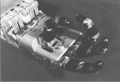
Figure 5.1: The Utah/MIT hand. (Photo courtesy of Sarcos, Inc.)

attached to a robot in an e cient fashion. While this e ectively extends the class of objects which can be lifted, it does not specifically address the fine motion problem.

In this chapter and the next, we investigate the use of multifingered robot hands as an alternative method for overcoming these di culties. A multifingered hand is a set of robots which is attached to the end of a larger robot arm for the purpose of manipulation. Since a robot hand is typically smaller than the robot to which it is attached, it is able to improve the overall accuracy of the robot. Further, the extra degrees of freedom in a multifingered hand make it possible to grasp a large class of objects with a single “end-e ector.”

The price of using a multifingered hand is the complexity of the overall system. A robot arm with a multifingered end-e ector has many degrees of freedom, complicating both the kinematic and dynamic analyses of the system. In particular, since the hand is in contact with the object being manipulated, we must study the kinematics and dynamics of mechanical systems with contact constraints. Additionally, the increased degrees of freedom of the system increase the di culty of planning a feasible grasp to perform a given task.

Because of the added complexity inherent in the use of robot hands, it is important to realize that a multifingered robot hand is not the answer to every manipulation problem. The use of custom end-e ectors can solve a large number of problems in such areas as manufacturing and materials

212