mls94-complete[1]

where all quantities are specified relative to a single base and tool frame. Equation (3.65) is called the structure equation (or loop equation) for the manipulator and introduces constraints between the possible joint angles of the manipulator. It is because of these constraints that we can control the end-e ector location by specifying only a subset of the joint variables: the other joint variables must take on values such that equation (3.65) is satisfied.

Since the joint variables are constrained by equation (3.65), the joint space for a parallel manipulator is not simply the Cartesian product of the individual joint spaces, as in the open-chain case. Rather, it is the subset Q′ Q which also satisfies equation (3.65). Determining the dimension of Q′, and hence the number of degrees of freedom for the parallel manipulator, requires careful inspection of the number of joints and links in the mechanism.

Let N be the number of links in the mechanism, g the number of joints, and fi the number of degrees of freedom for the ith joint. The number of degrees of freedom can be obtained by taking the total degrees of freedom for all of the links and subtracting the number of constraints imposed by the joints attached to the links. If all of the joints define independent constraints, the number of degrees of freedom for the mechanism is

Equation (3.66) is called Gruebler’s formula. Gruebler’s formula only holds when the constraints imposed by the joints are independent. For planar motions, Gruebler’s formula holds with 6 replaced by 3.

Although the forward kinematics of a parallel manipulator is complicated by the closed loop nature of the mechanism, the inverse problem is no more di cult than in the open-chain case. Namely, the inverse kinematics problem for a parallel manipulator is solved by considering the inverse problem for each open-chain mechanism which connects the ground to the end-e ector. This can be done using the methods presented in Section 3.

Velocity and force relationships

The velocity of the end-e ector of a parallel manipulator is related to the velocity of the joints of the manipulator by di erentiating the structure equation (3.65). This gives a Jacobian matrix for each chain:

133

where

Since the mechanism contains closed kinematic chains, not all joint velocities can be specified independently.

The manipulator Jacobian can be written in more conventional form by stacking the Jacobians for each chain:

This equation has a form very similar to one which we shall use in Chapter 5 to describe the kinematics of a multifingered grasp. Indeed, if we view each of the chains as grasping the end-e ector link via a prismatic or revolute joint, then a parallel manipulator is very similar to a multifingered hand grasping an object.

The relationship between joint torques and end-e ector forces for a parallel manipulator is more complicated than for an open-chain manipulator. The basic problem is that two or more chains can fight against each other and apply forces which cause no net end-e ector wrench. A set of joint torques which causes no net end-e ector wrench is called an internal force. We defer a discussion of internal forces until Chapter 5, where they arise naturally in the context of grasping.

Singularities

Determining the singularities of parallel mechanisms is more involved than it is for serial mechanisms. Consider a general parallel mechanism with k chains and let Θi denote the joint variables in the ith chain. The Jacobian of the structure equations has the form

We say that an end-e ector velocity is admissible at a configuration Θ =

˙

(Θ1, . . . , Θk) if there exist Θi which satisfy equation (3.69). The set of admissible velocities forms a linear space, since it is the intersection of the range spaces of Ji(θ), i = 1, . . . , k. Hence, we can define the rank of the structure equations, ρ, at a configuration Θ as the dimension of the space of admissible velocities,

where R(A) denotes the range space of the matrix A.

A parallel mechanism is kinematically singular at a point if the rank of the structure equations drops at that point. In this case, the tool loses

134

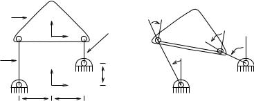
Figure 3.19: Four-bar linkage.

the ability to move instantaneously in some direction. This is analogous to our description of singularities in serial mechanisms. However, at this point we have not yet identified which joints in the mechanism are actuated and which are passive. If a parallel mechanism is fully actuated, then these are the only types of singularities that can occur. However, in most instances, only some of the joints of a parallel manipulator are actuated and this can lead to additional singularities. We call this second type of singularity an actuator singularity and give an example of it when we study the Stewart platform in Section 5.4.

5.3Four-bar linkage

To illustrate some of the concepts introduced above, we consider the four-bar linkage shown in Figure 3.19. The mechanism consists of three rigid bodies connected together by revolute joints. The links attached to the ground frame are called the input and output links, the rigid body which connects the input and output links is called the coupler. It is called a four-bar mechanism even though there are only three links, since historically the ground frame is considered to be the fourth link.

Four-bar linkages are usually studied in the context of mechanism synthesis. For example, we might try to find a mechanism such that the input and output links satisfy a given functional relationship, creating a type of mechanical computer. Alternatively, one might wish to design the mechanism so that a point on the coupler traces a specified path or passes through a set of points. Many other variations exist, but for all of these problems one tries to choose the kinematic parameters which describe the mechanism—the lengths of the links, shape of the coupler, location of the joints—so that a given task is performed. In this section, we bypass the synthesis problem and concentrate on kinematic analysis of a given mechanism.

135

The number of degrees of freedom of a four-bar mechanism is given by Gruebler’s formula:

The fact that there is only one degree of freedom helps explain the terminology of the input and output links. Note that we used the planar version of Gruebler’s formula to calculate the mobility of the mechanism. A quick calculation shows that the spatial version of the formula gives F = 6(3 − 4) + 4 = −2 (!). We leave the resolution of this apparent paradox as an exercise.

To write the structure equations, we must first assign base and tool frames and choose a reference configuration. The tool and base frames are assigned as shown in the figure. We choose the reference configuration (θ = 0) to be the configuration shown in Figure 3.19a. Note that this is not the usual reference configuration if we had considered each of the kinematic chains as independent two-link robots. However, it will be convenient to have the reference configuration satisfy the kinematic constraints and hence we define the angles as shown in Figure 3.19b. With respect to this configuration, the structure equations have the form

Note that in the plane this gives three constraints in terms of four variables, leaving one degree of freedom as expected.

The twists can be calculated using the formulas for twists in the plane derived in the exercises at the end of Chapter 2. In particular, a revolute joint in the plane through a point q = (qx, qy ) is described by a planar

ξ = −qx R3.

1

This yields

Expanding the product of exponentials formula gives

−r − l1 sin θ11 + r cos(θ11 + θ12) = x = r − l2 sin θ21 − r cos(θ21 + θ22) l1 cos θ11 + r sin(θ11 + θ12) = y = h + l2 cos θ21 − r sin(θ21 + θ22)

θ11 + θ12 = φ = θ21 + θ22

136

where φ is the angle the tool frame makes with the horizontal. From the form of this equation, it is clear that solving for the forward kinematics is a complicated task, though it turns out that in many cases it can be done in closed form.

The Jacobian of the structure equation has the form

To calculate the individual columns of the Jacobian, we write the twists at the current configuration of the manipulator. Thus,

This gives the velocity constraints on the system. Since the individual Jacobians for each chain only have two columns, it is clear that the dimension of the space of admissible velocities is at most two. To examine the mobility more closely, we rearrange the Jacobian to isolate the actuated and passive joints.

Suppose we take θ = θ11 as the actuated joint and let α = (θ12, θ21, θ22) represent the passive joints. The Jacobian of the structure equation can

(this type of rearrangement works only in the special case where we have two serial chains or a single kinematic loop). The form of this equation suggests that if we specify the velocity of the actuated joint θ, then we can solve for the velocity of the passive joints if the right-hand side of equation (3.71) is nonsingular.

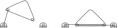
The right-hand side of equation (3.71) corresponds to the twists generated by three parallel, revolute joints. We know from our study of singularities of twists that if the three axes are coplanar in addition to being parallel, then the twists are linearly dependent. In the planar case, this means that if the passive joints are collinear, then the right-hand side of equation (3.71) loses rank and the mechanism may not be able to move. However, this condition is not su cient since it may happen that ξ11 is in the range of {ξ12′ , ξ21, ξ22′ } even though they are singular. These two di erent situations are shown in Figure 3.20. Note that switching the role of the input and output links changes the singular configurations of the mechanism. For example, the singularity shown in Figure 3.20a is only a singularity if the left-hand link is chosen as the input link (since this choice gives three collinear passive joints).

The configuration shown in Figure 3.20b is known as an uncertainty configuration in the kinematics literature. In this case, it is actually

137

active joint

Figure 3.20: Potential singular configurations for four-bar mechanisms.

possible for the mechanism to move instantaneously in two independent directions. Examining the structure equations, we see that

represent two independent, instantaneously admissible velocities. These two independent velocities exist only if the mechanism is perfectly aligned and hence uncertainty configurations rarely occur in practice.

5.4Stewart platform

Another common example of a parallel mechanism is the Stewart platform, an example of which is shown in Figure 3.21. The mechanism consists of two rigid bodies, connected by a set of prismatic joints. Each prismatic joint is connected to the rigid body by a spherical joint, allowing complete rotational motion. Only the prismatic joints are actuated.

Stewart platforms are commonly used in aircraft flight simulators to move an aircraft cockpit along the motion indicated by the (simulated) dynamics of the system. Although the concept of a Stewart platform is quite old (it was studied by Stewart in the 1950s [111]), it is only recently that the kinematics for a general Stewart platform have been solved in complete generality.

In order to write the structure equation for a Stewart platform, we must first take a slight detour and discuss the modeling of a spherical joint. For the manipulators we have considered previously, we have always modeled a spherical joint as three revolute joints intersecting at a

138

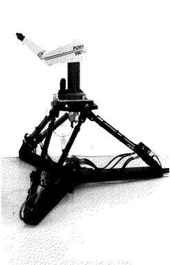
Figure 3.21: A Stewart platform with a PUMA robot attached. (Photo courtesy of Steve Dubowsky, MIT)

point. This made physical sense since this is how most actuated spherical wrists are built. However, spherical wrists always have singularities when any two of the axes become parallel (it can be shown that this will always happen for some choice of joint angles). In a Stewart platform, the spherical joints are completely passive and hence will never become singular. This requires that we define spherical joints slightly di erently than spherical wrists.

The rigid motion generated by a spherical joint has the form

where R is a free parameter and q is the location of the center of the wrist. Similarly, the velocity of a spherical joint has the form

139

where ω is a free parameter (the velocity). To cast this equation into a more useful framework, we rewrite V s as

where ei is the ith unit vector in R3. Notice that the columns of the matrix which defines V s are never linearly dependent.

We can now write the structure equations for the Stewart platform. Let gsi (Rsi ) represent the orientation of the ith spherical joint attached to the base and gti (Rti ) represent the ith spherical joint attached to the tool. Then, the structure equation for the Stewart platform is given by

where ξi and θi model the motion of the ith prismatic joint.

Solving the forward kinematics for a Stewart platform is a very di - cult problem due to the large number and complicated form of the constraints. Abstractly, given the length of the links, we can solve the structure equations to find the orientations of the ball and socket joints and then determine the configuration of the tool frame. As the problem has been specified here, there is an extra degree of freedom in each link corresponding to rotation of the prismatic joint about its own axis. This further complicates the forward kinematics problem.

The inverse kinematics problem for the Stewart platform is remarkably simple. Given the desired configuration of the platform, we find the locations of the pivot points and solve for the distance between each base and the appropriate pivot. Let qsi be the location of the ith pivot point on the base and qti be the location of the tool pivot point (written relative to the base and tool frames, respectively). Then, the extension of the prismatic joints is given by

θi = kqsi − gstqti k.

It is possible to derive this result in a manner similar to that used in solving the subproblems of Section 3; but in this case, the solution is obvious from the geometry of the manipulator.

We may now study the mobility of the Stewart platform by calculating the Jacobian of the structure equation. Taking the Jacobian of

140

It can be shown that the Jacobian matrices are never singular as long as θi is nonzero (see Exercise 22). Hence, all tool velocities are admissible.

However, an interesting problem occurs when the tool frame and base frame are coplanar. In this case, the actuated joints can only generate forces in the plane, and hence the mechanism cannot resist (or apply) nonplanar forces or torques. Note that the mechanism is still not kinematically singular: the joints can accommodate any motion of the tool frame. However, the actuated joints cannot generate the wrenches necessary to actually achieve any motion. This is an example of the second class of singularity that was mentioned previously. We call this type of singularity an actuator singularity since it corresponds to a failure of the actuated joints to be able to generate arbitrary wrenches in the tool frame. This type of singularity is very closely related to the failure of the force-closure conditions which occur in grasping.

A geometric interpretation of this singularity in the Stewart platform can be obtained by noting that the system of wrenches which can be applied to the tool frame is given by the set of all zero-pitch (pure force) wrenches generated by the actuated joints through the points qti . Since the prismatic joints generate zero-pitch wrenches, we can use the previously derived examples of singularities of zero-pitch screws to locate some of the singularities of the Stewart platform. In this context, when the base and tool frames are coplanar, we get a singularity because we have four (actually six) coplanar, zero-pitch screws. A separate singularity occurs whenever two of the prismatic joints are collinear.

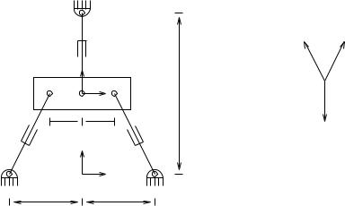
Example 3.18. Singularities for a planar Stewart platform

Consider the planar parallel mechanism shown in Figure 3.22. Three actuated prismatic joints are used to control the position and orientation of the platform. The revolute joints at the end of each link are passive. Kinematically, this mechanism shares some of the properties of the Stewart platform.

We concentrate on the singularities of the mechanism. As with the Stewart platform, it can be shown that there are no kinematic singularities where the dimension of the space of achievable velocities drops rank (it is always three). Since the actuated joints are all prismatic, the

141

R R

Figure 3.22: A planar version of the Stewart platform.

wrenches generated by the joints correspond to zero-pitch screws. In the plane, it can be shown that three zero-pitch screws intersecting at a point are singular. This is exactly the configuration in which the mechanism is drawn in Figure 3.22 (see the wrench diagram to the right).

Hence, in this configuration, it is not possible for the mechanism to generate pure torques around the point of common intersection. This is clear if we write down the wrenches relative to a coordinate frame attached at the intersection point. In this set of coordinates, we have

where vi is the direction of the ith prismatic axis and fi is the force exerted by the ith actuator. It is clear that we cannot generate a pure torque around the intersection point since

142