FIGURE 9-9

Load step transient and stability limit of synchronous machine.

be exceeded under any condition, including those that can be encountered during transients. For example, if a sudden load step is applied to the machine initially operating in a steady state at load power angle δ1 (Figure 9-9), the rotor power angle would increase from δ1 to δ2 corresponding to the new load that it must supply. This takes some time depending on the electromechanical inertia of the machine. No matter how short or long it takes, the rotor inertia and the electromagnetic restraining torque will set the rotor in a mass-spring type of oscillatory mode, swinging the rotor power angle beyond its new steady state value. If the power angle exceeds 90° during this swing, the machine stability and the power generation are lost. For this reason, the machine can be loaded only to the extent that even under the worst-case step load, planned or accidental, or during all possible faults, the power angle swing will remain below 90° with sufficient margin. This limit on loading the machine is called the transient stability limit.

Equation 9-5 shows that the stability limit at given voltages can be increased by designing the machine with low synchronous reactance Xs , which is largely made of the stator armature reaction component.

9.4Commercial Power Plants

The commercial power plants using the solar thermal system are being explored in a few hundred MWe capacity. Based on the Solar II power plant operating experience, the design studies made by the National Renewable Energy Laboratory for the U.S. Department of Energy have estimated the

© 1999 by CRC Press LLC

FIGURE 12-8

Integrated power connection and control unit for wind-pv-battery hybrid system. (Source: World Power Technologies, Duluth, Minnesota. With permission.)

Factories and hospitals have considered the fuel cell to replace the diesel generator in the uninterruptible power system. Electric utility companies are considering the fuel cell for meeting the peak demand and for load leveling between the day and night and during the week.

The fuel cell is an electrochemical device that generates electricity by chemical reaction without altering the electrodes or the electrolyte materials. This distinguishes the fuel call from the electrochemical batteries. The concept of the fuel cell is the reverse of the electrolysis of water, in which the hydrogen and oxygen are combined to produce electricity and water. The fuel cell is a static device that converts the chemical energy directly into electrical energy. Since fuel cell bypasses the thermal-to-mechanical conversion, and since its operation is isothermal, the conversion efficiency is not Carnot-limited. This way, it differs from the diesel engine.

The fuel cell, developed as an intermediate-term power source for space applications, was first used in a moon buggy and continues to be used to power NASA’s space shuttles. It also finds other niche applications at present. Providing electrical power for a few days or a few weeks is not practical using the battery, but is easily done with the fuel cell.

The basic constructional features of the fuel cell are shown in Figure 12-9. The hydrogen ‘fuel’ is combined with oxygen of the air to produce electricity. The hydrogen, however, does not burn as in the internal combustion engine, rather it produces electrically by an electrochemical reaction. Water and heat are the byproducts of this reaction if the fuel is pure hydrogen. With the natural gas, ethanol or methanol as the source of hydrogen, the byproducts include carbon dioxide, and traces of carbon monoxide, hydrocarbons and nitrogen oxides. However, they are less than 1 percent of those emitted by the diesel engine. The superior reliability with no moving parts is an additional benefit of the fuel cell over the diesel generator. Multiple fuel cells

© 1999 by CRC Press LLC

FIGURE 12-9

Fuel cell principle: hydrogen and oxygen in, electrical power and water out.

stack up in series-parallel combinations for the required voltage and current, just as the electrochemical cells do in the battery.

The low temperature (250°C) fuel cell is now commercially available from several sources. It uses phosphoric acid as the electrolytic solution between the electrode plates. A typical low temperature fuel cell with a peak power rating of 200 kW costs under $1,800 per kW at present, which is over twice the cost of the diesel engine. The fuel cell price, however, is falling with new developments being implemented every year.

The high temperature fuel cell has a higher power generation capacity per kilogram at a relatively high cost, limiting the use in special applications at present. Solid oxide, solid polymer, molten carbonate, and proton membrane exchange fuel cells in this category are being developed. The industry interest in such cells is in large capacity for use in a utility power plant. The Fuel Cell Commercialization Group in the U.S.A. recently field-tested molten carbonate direct-fuel cells for 2 MW utility-scale power plants. The test results were a qualified success. Based on the results, a commercial plant is being designed for a target date of operation by the year 2000.

Solid oxide fuel cells of several different designs, consisting of essentially similar materials for the electrolyte, the electrodes, and the interconnections, are being investigated worldwide. Most success to date has been achieved with the tubular geometry being developed by the Westinghouse Electric

© 1999 by CRC Press LLC

FIGURE 12-10

Air electrode supported type tubular solid oxide fuel cell design. (Courtesy of Westinghouse Electric Company, A Division of CBS Corporation, Pittsburgh, PA. Reprinted with permission.)

Corporation in the U.S.A. and Mitsubishi Heavy Industries in Japan. The cell element in this geometry consists of two porous electrodes separated by a dense oxygen ion-conducting electrolyte as depicted in Figure 12-10.4 It uses ceramic tube operating at 1,000°C. The fuel cell is an assembly of such tubes. SureCELL™ (Trademark of Westinghouse Electric Corporation, Pittsburgh, Pennsylvania) is a solid oxide high temperature tubular fuel cell shown in Figure 12-11. It is being developed for multi-megawatt combined cycle gas turbine and fuel cell plants and targeted for distributed power generation and cogeneration plants of up to 60 MW capacity. It fits well for utility scale wind and photovoltaic power plants. Inside SureCELL, natural gas or other fuels are converted to hydrogen and carbon monoxide by internal reformation. No external heat or stream is needed. Oxygen ions produced from an air stream react with the hydrogen and carbon monoxide to generate electric power and high temperature exhaust gas.

Because of the closed-end tubular configuration, no seals are required and relative cell movement due to differential thermal expansions is not restricted. This enhances the thermal cycle capability. The tubular configuration solves many of the design problems facing other high temperature fuel cells. The target for the SureCELL development is to attain 75 percent overall efficiency, compared to 60 percent possible using only the gas turbine (Figure 12-12). Environmentally, the solid oxide fuel cell produces much lower CO2, NOx and virtually zero SOx compared with other fuel cell technologies.

During the eight years of failure-free steady state operation of early prototypes, these cells were able to maintain the output voltage within 0.5 percent per 1,000 hours of operation. The second generation of the Westinghouse fuel cell shows voltage degradation of less then 0.1 percent per 1,000 hours of operation, with life in tens of thousands of hours of operation. The SureCELL prototype has been tested for over 1,000 thermal cycles with

© 1999 by CRC Press LLC

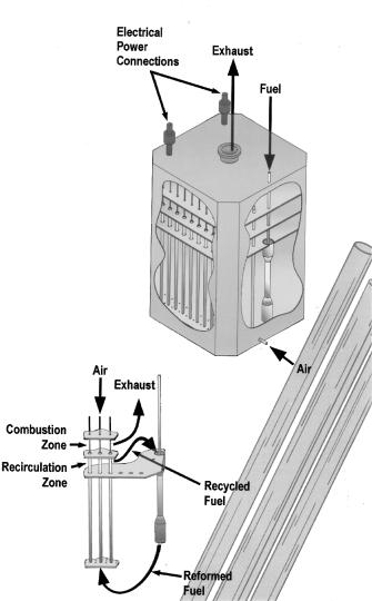
FIGURE 12-11

Seal-less solid oxide fuel cell power generator. (Courtesy of Westinghouse Electric Company, A Division of CBS Corporation, Pittsburgh, PA. Reprinted with permission.)

zero performance degradation, and 12,000 hours of operation with less then 1 percent performance degradation.

The transient electrical performance model of the fuel cell includes electrochemical, thermal, and mass flow elements that affects the electrical output.5 Of primary interest is the electrical response of the cell to a load change. To design for the worst case, the performance is calculated under both the constant reactant flow and the constant inlet temperature.

© 1999 by CRC Press LLC

FIGURE 12-12

Natural gas power generation system efficiency comparison. (Courtesy of Westinghouse Electric Company, A Division of CBS Corporation, Pittsburgh, PA. Reprinted with permission.)

The German-American car-manufacturer Daimler-Chrysler and Ballard Power Systems of Canada are developing the solid polymer fuel cell for automobiles as an alternative to the battery-powered vehicles. Their target is to sell the first commercial fuel cell powered car by the year 2004.

12.4.3Mode Controller

The overall system must be designed for a wide performance range to accommodate the characteristics of the diesel generator (or fuel cell), the wind generator, and the battery. As and when needed, switching to the desired mode of generation is done by the mode controller. Thus, the mode controller is the central monitor and controller of the hybrid systems. It houses the microcomputer and software for the source selection, the battery management, and load shedding strategy. The mode controller performs the following functions:

•monitors and controls the health and state of the system.

•monitors and controls the battery state-of-charge.

•brings up the diesel generator when needed, and shuts off when not needed.

•sheds low priority loads in accordance with the set priorities.

The battery comes on-line by automatic transfer switch, which takes about 5 ms to connect to the load. The diesel, on the other hand, is generally brought

© 1999 by CRC Press LLC

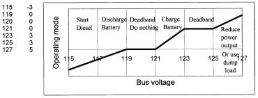
FIGURE 12-13

Mode controller deadbands eliminates the system chatter.

on-line, manually or automatically after going through the preplanned strategy algorithm. Even with automatic transfer switches, the diesel generator takes a long time to come on-line. Typically, this delay time is approximately 20 seconds.

The mode controller is designed and programmed with deadbands to avoid change over of the sources for correcting small variation on the bus voltage and frequency. The deadbands avoid chatters in the system. Figure 12-13 is an example of 120 volts hybrid system voltage-control regions. The deadbands are along the horizontal segments of the control line.

As a part of the overall system controller, the mode controller may incorporate the maximum power extraction algorithm. The dynamic behaviors of the closed-loop system, following common disturbances such as insolation changes due to cloud, wind fluctuation, sudden load changes and short circuit faults, are taken into account in a comprehensive design.6

12.4.4Load Sharing

Since the wind, pv, battery, and diesel (or fuel cell) in various combinations, operate in parallel, the load sharing between them is one of the key design aspects of the hybrid system. For example, in the wind/diesel hybrid system (Figure 12-14), the electrical properties of the two systems must match so that they share load in proportion to their rated capacities.

For determining the load sharing, the two systems are first reduced to their respective Thevenin equivalent circuit model, in which each system is represented by its internal voltage and the series impedance. This is shown in Figure 12-14. The terminal characteristics of the two generators are then given by the following:

E1 = E01 − I1 Z1

(12-1)

E2 = E02 − I2 Z2

where subscripts 1 and 2 represent system 1 and 2 respectively, and

© 1999 by CRC Press LLC

FIGURE 12-14

Thevenin’s equivalent model of two sources in hybrid power system.

Eo = internally generated voltage

Z = internal series impedance

E = terminal voltage of each system

If the two generators are connected together, their terminal voltages E1

and E2 must be equal to the bus voltage Vbus. Additionally, the sum of the component loads I1 and I2 must be equal to the total load current IL. Thus,

the conditions imposed by the terminal connection are as follows:

E1 = E2 = Vbus

These imposed conditions, along with the machines internal characteristics Eo and Z, would determine the load sharing I1 and I2. The loading on individual generators is determined algebraically by solving the two simultaneous equations for the two unknowns, I1 and I2. Alternatively, the solution is found graphically as shown in Figure 12-15. In this method, E versus I characteristics of the two power systems are first individually plotted on the two sides of the current axis (horizontal). The distance between the two voltage axes (vertical) is kept equal to the total load current IL. The electrical generators will share the load such that their terminal voltages are exactly equal, the condition imposed by connecting them together at the bus. This condition is met at the point of intersection of the two load lines. The point P in the figure, therefore, settles the bus voltage and the load sharing. The current I1 and I2 in the two generators are then read from the graph.

Controlling the load sharing requires controlling the E versus I characteristic of the machines. This may be easy in case of the separately excited DC or the synchronous generator used with the diesel engine. It is, however, difficult in case of the induction machine. Usually the internal impedance Z is fixed once the machine is built. Care must be exercised in the hybrid design

© 1999 by CRC Press LLC

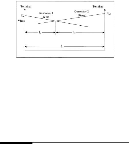
FIGURE 12-15

Graphical determination of load shared by two sources in hybrid power system.

to make sure that sufficient excitation control is built in for the desired load sharing between the two sources.

The load sharing strategy can vary depending on the priority of loads and the cost of electricity from alternative sources. In a wind-diesel system, for example, diesel electricity is generally more expensive than wind (~25 versus 5 cents per kWh). Therefore, all priority-1 (essential) loads are met first by wind as far as possible and then by diesel. If the available wind power is more than priority-1 loads, wind supplies part of priority-2 loads and the diesel is not run. If the wind power now fluctuates on the down side, the lower priority loads are shed to avoid running the diesel. If wind power drops further to cut into the priority-1 load, the diesel is brought on-line again. Water pumping and heater loads are examples of priority-2 loads.

12.5 System Sizing

For determining the required capacity of the stand-alone power system, estimating the peak load demand is only one aspect of the design. Estimating the energy required over the duration selected for the design is the first requirement for the system sizing.

12.5.1Power and Energy Estimates

The system sizing starts with compiling a list of all loads that are to be served. Not all loads are constant. Time-varying loads are expressed in peak watts they consume and the duty ratio. The peak power consumption is used in determining the wire size for making a connection to the source.

© 1999 by CRC Press LLC

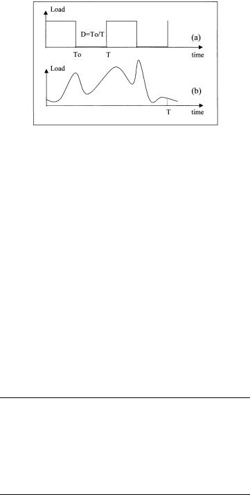
FIGURE 12-16

Duty ratio and peak power of intermittent loads.

The duty ratio is used in determining the contribution of individual load in the total energy demand. If the load has clean on-off periods as shown in Figure 12-16(a), then the duty ratio D is defined as D = To/T, where To is the time the load is on and T is the period of repetition. For irregularly varying loads shown in (b), the duty ratio is defined as the actual energy consumed in one period over the peak power times the period, i.e.:

The peak power consumption and the duty ratio of all loads are compiled, the product of the two is the actual share of the energy requirement of that load on the system during one repetition period. If there are distinct intervals in the period, say between the battery discharge and charge intervals, then the peak power and the duty ratio of each load are computed over the two intervals separately. As a simple example of this in a solar power system, one interval may be from 8 A.M. to 6 P.M. and the other from 6 P.M. to 8 A.M. The power table is then prepared as shown in Table 12-2.

TABLE 12-2

Power and Energy Compilation Table for Energy Balance Analysis

Total Battery Discharge Required = Σ Eb watts-hours

© 1999 by CRC Press LLC

TABLE 12-3

NEC® Demand Factors (Adapted from National Electrical Code® Handbook, 7th Edition, 1996, Table 220-32)

In a community of homes and businesses, not all connected loads draw power simultaneously. The statistical time staggering in their use times results in the average power capacity requirement of the plant significantly lower than the sum of the individually connected loads. The National Electrical Code® provides factors for determining the average community load in normal residential and commercial areas (Table 12-3). The average plant capacity is then determined as follows:

Required power system capacity = NEC® factor from Table 12-3 × Sum of connected loads.

12.5.2Battery Sizing

The battery Ah capacity required to support the load energy requirement of Ebat as determined using a method of Table 12-2 or equivalent:

The following example illustrates the use of this formula to size the battery. Suppose we want to design a battery for a stand-alone power system, which charges and discharges the battery from 110 volts DC solar array. For the

© 1999 by CRC Press LLC

DC-DC buck converter that charges the battery, the maximum available battery-side voltage is 70 volts for it to work efficiently in the PWM mode. For the DC-DC boost converter discharging the battery, the minimum required battery voltage is 45 volts. Assuming that we are using NiMH battery, the cell voltage can vary from 1.55 when fully charged to 1.1 when drained to the maximum allowable DOD. Then, the number of cells needed in the battery is less than 70/1.55 = 45 cells and more than 45/1.1 = 41. Thus, the number of cells required in the battery from the voltage considerations is between 41 and 45. It is generally more economical to use fewer cells of higher capacity than more lower-capacity cells. We, therefore, select 41 cells in the battery design.

Now again for an example, let us assume that the battery is required to discharge 2 kW load for 14 hours (28,000 Wh) every night for five years before replacement. The life requirement is, therefore, 5 365 = 1,825 cycles of deep discharge. For the NiMH battery, the cycle life at full depth of discharge is 2,000. Since this is greater than the 1,825 cycles required, we can fully discharge the battery every night for five years. If the discharge efficiency is 80 percent, the average cell discharge voltage is 1.2 V, and we desire three batteries in parallel for reliability, each battery Ah capacity calculated from the above equation is as follows:

Three batteries, each having 41 series cells of 237 Ah capacity, therefore, will meet the system requirement. Margin must be allowed to account for the uncertainty in estimating the loads.

12.5.3pv Array Sizing

The basic tenet in sizing the stand-alone “power system” is to remember that it is really the stand-alone “energy system.” It must, therefore, maintain the energy balance over the specified period. The energy drained during lean times must be made up by the positive balance during the remaining time of the period. A simple case of a constant load on the pv system using solar arrays perfectly pointing toward the sun normally for 10 hours of the day is shown in Figure 12-17 to illustrate the point. The solar array is sized such that the two shaded areas on two sides of the load line must be equal. That is, the area oagd must be equal to the area gefb. The system losses in the round trip energy transfers, e.g., from and to the battery, adjust the available load to a lower value as shown by the dotted line.

In general, the stand-alone system must be sized so as to satisfy the following energy balance equation over one period of repetition.

© 1999 by CRC Press LLC

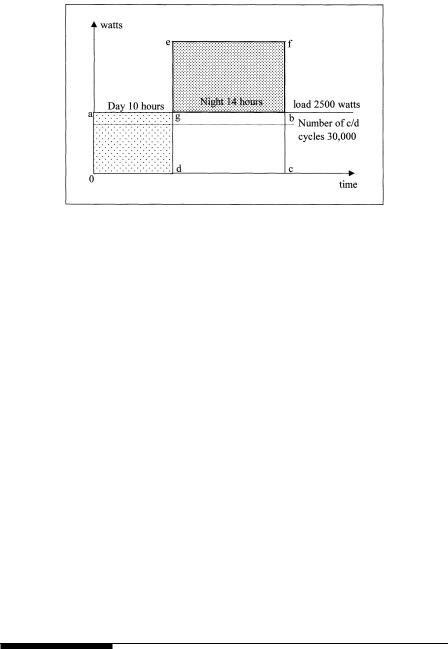
FIGURE 12-17

Energy balance analysis over one load cycle.

Or, in discrete time intervals of constant load and source power:

12.6 Wind Farm Sizing

In a stand-alone wind farm, selecting the number of towers and the battery size depend on the load power availability requirement. A probabilistic

© 1999 by CRC Press LLC

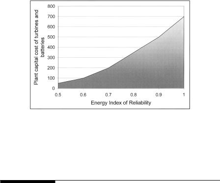
FIGURE 12-19

Relative capital cost versus EIR with different numbers of wind turbines and battery sizes.

Setting unnecessarily high EIR requirement can make the project uneconomical. For that reason, the Energy Index of Reliability must be set after a careful optimization of the cost and the consequences of not meeting the load requirement during some portion of the time period.

References

1.“Institute of Solar Energy and Technology Annual Report,” Kassel, Germany, 1997.

2.Wang, L. and Su, J. 1997. “Dynamic performance of an isolated self-excited induction generator under various load conditions,” IEEE Power Engineering Paper No. PE-230-EC-1-09, 1997.

3.Bonarino, F., Consoli, A., Baciti, A., Morgana, B. and Nocera, U. 1998. “Transient analysis of integrated diesel-wind-photovoltaic generation systems,” IEEE Paper No. PE-425-EC-104, July 1998.

4.Singhal, S. C. 1996. “Status of solid oxide fuel cell technology,” Proceedings of the 17th Risø International Symposium on Material Science, High Temperature Electrochemistry, Ceramics and Metals, Roskilde, Denmark, Sept. 1996.

5.Hall, D. J. and Colclaser, R. G. 1998. “Transient modeling and simulation of a tubular solid oxide fuel cell,” IEEE Paper No. PE-100-EC-004, July 1998.

6.Abdin, E. S., Asheiba, A. M., and Khatee, M. M. 1998. “Modeling and optimum controllers design for a stand-alone photovoltaic-diesel generating unit,” IEEE Paper No. PE-1150-0-2, 1998.

7.Baring-Gould, E. I. 1996. “Hybrid2, The hybrid system simulation model user manual,” NREL Report No. TP-440-21272, June 1996.

© 1999 by CRC Press LLC

13

Grid-Connected System

The wind and photovoltaic power systems have made a successful transition from small stand-alone sites to large grid-connected systems. The utility interconnection brings a new dimension in the renewable power economy by pooling the temporal excess or the shortfall in the renewable power with the connecting grid. This improves the overall economy and the load availability of the renewable plant; the two important factors of any power system. The grid supplies power to the site loads when needed, or absorbs the excess power from the site when available. One kWh meter is used to record the power delivered to the grid, and another kWh meter is used to record the power drawn from the grid. The two meters are generally priced differently.

Figure 13-1 is a typical circuit diagram of the grid-connected photovoltaic power system. It interfaces with the local utility lines at the output side of the inverter as shown. A battery is often added to meet short term load peaks. In the United States, the Environmental Protection Agency sponsors gridconnected pv programs in urban areas where wind towers would be impractical. In recent years, large building-integrated photovoltaic installations have made significant advances by adding the grid-interconnection in the system design. Figure 13-2 shows the building-integrated pv system on the roof of the Northeastern University Student Center in Boston, MA. The project was part of the EPA PV DSP Program. The system produces 18 kW pv power and is connected to the grid. In addition, it collects sufficient research data using numerous instruments and computer data loggers. The vital data are sampled every 10 seconds, and then are averaged and stored every 10 minutes. The incoming data includes information about the air temperature and wind speed. The performance parameters include the DC voltage and current generated by the pv roof, and the AC power on the inverter output side.

In the United Kingdom, a 390 square meter building-integrated pv system has been in operation since 1995 at the University of Northumbria, Newcastle (Figure 13-3). The system produces 33,000 kWh electricity per year and is connected to the grid. The pv panels are made of monocrystalline cells with the photoconversion efficiency of 14.5 percent.

On the wind side, most grid-connected systems are large utility-scale power plants. A typical equipment layout in such plants is shown in Figure 13-4. The wind generator output is at 480 volts AC, which is raised

© 1999 by CRC Press LLC

FIGURE 13-1

Electrical schematic of the grid-connected photovoltaic system.

FIGURE 13-2

18 kW grid-connected pv system on the Northeastern University Student Center in Boston, MA. (Source: ASE Americas, Billerica, Massachusetts. With permission.)

to an intermediate level of 21 kV by a pad-mounted transformer. An overhead transmission line provides the link to the site substation, where the voltage is raised again to the grid level. The site computer, sometimes using mulitplexer and remote radio links, controls the wind turbines in response to the wind conditions and the load demand.

© 1999 by CRC Press LLC

FIGURE 13-3

Grid-connected pv system at the University of Northumbria, Newcastle, U.K. The 390 square meter monocrystalline modules produce 33,000 kWh per year. (Source: Professional Engineer, Publication of the Institution of Mechanical Engineer’s, London. With permission.)

© 1999 by CRC Press LLC

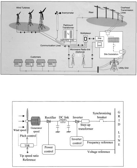
FIGURE 13-4

Electrical component layout of the grid-connected wind power system. (Source: AWEA/IEA/ CADDET Technicla Brochure, 1995.)

FIGURE 13-5

Electrical schematic of the grid-connected variable speed wind power system.

Large wind systems being installed now tend to have the variable-speed design. The power schematic of such a system is shown in Figure 13-5. The variable-frequency generator output is first rectified into DC, and then inverted into a fixed-frequency AC. Before the inversion, the rectifier harmonics are filtered out from the DC by the inductor and capacitors. The frequency reference for the inverter firing and the voltage reference for the rectifier phase-angle control are taken from the grid lines. The optimum reference value of the tip-speed ratio is stored and continuously compared

© 1999 by CRC Press LLC

with the value computed from the measured speeds of the wind and the rotor. The turbine speed is accordingly changed to assure maximum power production at all times.

13.1 Interface Requirements

Both the wind and the pv systems interface the grid at the output terminals of the synchronizing breaker at the output end of the inverter. The power flows in either direction depending on the site voltage at the breaker terminals. The fundamental requirements on the site voltage for interfacing with the grid are as follows:

•the voltage magnitude and phase must equal to that required for the desired magnitude and direction of the power flow. The voltage is controlled by the transformer turn ratio and/or the rectifier/inverter firing angle in a closed-loop control system.

•the frequency must be exactly equal to that of the grid, or else the system will not work. To meet the exacting frequency requirement, the only effective means is to use the utility frequency as a reference for the inverter switching frequency.

•in the wind system, the synchronous generators of the grid system supply magnetizing current for the induction generator.

The interface and control issues are similar in many ways between both the pv and the wind systems. The wind system, however, is more involved since the electrical generator and the turbine with large inertia introduce certain dynamic issues not applicable in the static pv system. Moreover, wind plants generally have much greater power capacity than the pv plants. For example, many wind plants that have been already installed around the world have capacity in tens of MW each. The newer wind plants in the hundreds of MW capacity are being installed and more are planned.

13.2 Synchronizing with Grid

The synchronizing breaker in Figures 13-1 and 13-5 has internal voltage and phase angle sensors to monitor the site and grid voltages and signal the correct instant for closing the breaker. As a part of the automatic protection circuit, any attempt to close the breaker at an incorrect instant is rejected by the breaker. Four conditions which must be satisfied before the synchronizing switch will permit the closure are as follows:

© 1999 by CRC Press LLC

•the frequency must be as close as possible with the grid frequency, preferably about one-third of a hertz higher.

•the terminal voltage magnitude must match with that of the grid, preferably a few percent higher.

•the phase sequence of the two three-phase voltages must be the same.

•the phase angle between the two voltages must be within 5 degrees.

Taking the wind power system as an example, the synchronizing process specifically runs as follows:

1.With the synchronizing breaker open, the wind power generator is brought up to speed using the machine in the motoring mode.

2.Change the machine into the generating mode, and adjust the controls such that the site and grid voltages match to meet the above requirements as close as possible.

3.The match is monitored by the synchroscope or three synchronizing lamps, one in each phase (Figure 13-6). The voltage across the

FIGURE 13-6

Synchronizing circuit using three synchronizing lamps or the synchroscope.

© 1999 by CRC Press LLC

lamp in each phase is the difference between the renewable site voltage and the grid voltage at any instant. When the site and the grid voltages are exactly equal in all three phases, all three lamps will be dark. However, it is not enough for the lamps to be dark at any one instant. They must remain dark for a long time. This condition which will be met only if the generator and the grid voltages have nearly the same frequency. If not, one set of the two three-phase voltages will rotate faster relative to the other, and the phase difference between the two voltages will light the lamps.

4.The synchronizing breaker is closed if the lamps remain dark for 1⁄4 to 1⁄2 second.

Following the closure, any small mismatch between the site voltage and the grid voltage will circulate the inrush current between the two such that the two systems will come to perfect synchronous operation.

13.2.1Inrush Current

The small unavoidable difference between the site and the grid voltages will result in an inrush current to flow between the site and the grid. The inrush current eventually decays to zero at an exponential rate that depends on the internal resistance and inductance. The initial magnitude of this current in the instant the circuit breaker is closed depends on the degree of mismatch between the two voltages. It is not all bad, as it produces the synchronizing power which acts to bring the two systems in synchronous lock. However, it produces a mechanical torque step, setting up the electromechanical oscillations before the two machines come into synchronism and get locked with each other. The magnitude of the inrush current is calculated as follows:

Let ∆V be the difference between the site voltage and the grid voltage at the closing instant due to any reason. Since this voltage is suddenly applied on the system, the resulting inrush current is determined by the subtransient reactance of the machine Xd″. That is as follows:

The inrush current is primarily reactive, as is solely determined by Xd″. Its magnitude is kept within the allowable limit, else the thermal or mechanical damage may result.

The synchronizing power produced by the inrush current brings the wind system and the grid in synchronism after the oscillations decay out. Once synchronized, the generator has a natural tendency to remain in synchronism with the grid, although it can fall out of synchronization if excessive load is extracted, large load steps are applied, or during system faults. Small perturbation swings in the load angle decay out over a time, restoring the

© 1999 by CRC Press LLC

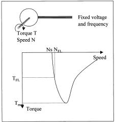
FIGURE 13-7

Resilience in the torque versus speed characteristic of induction generator.

synchronous condition. The magnitude of the restoring power, also known as the synchronizing power, is highest if the machine is running at no load, and is zero if it is running at its steady state stability limit.

13.2.2Synchronous Operation

Once synchronized, the voltage and frequency of the wind system need to be controlled. When the induction generator is directly connected to the grid, the grid serves as the frequency reference for the generator output frequency. The grid also acts as the excitation source supplying the reactive power. Since the torque versus speed characteristic of the induction generator has a steep slope near zero slip (Figure 13-7), the speed of the wind turbine remains approximately constant within a few percentages. Higher load torque is met by increased slip up to a certain point (Qm), beyond which the generator becomes unstable. If the load torque is immediately reduced, the generator will return to the stable operation. From the operating point of view, the induction generator is softer, as opposed to the relatively stiff operation of the synchronous generator, which works at an exact constant speed or falls out of stability.

If the synchronous generator is used, as in wind farms installed in California in the 1980s, the voltage is controlled by controlling the rotor field excitation current. The frequency control, however, is not required on a continuous basis. Once synchronized and connected with the lines, the synchronous generator has an inherent tendency to remain in synchronous lock with the grid. Only during transients and system faults, the synchronism can be lost. In such cases the generator must be resynchronized.

© 1999 by CRC Press LLC

In the variable-speed induction generator system using the inverter at the interface, the inverter gate signal is derived from the grid voltage to assure synchronism. The inverter stability depends a great deal on the design. For example, with line commutated inverter, there is no stability limit. The power limit in this case is the steady state load limit of the inverter with any shortterm overload limit.

13.2.3Load Transient

During steady state operation, if the renewable power system output is fully or partially lost, the grid will pick up the area load. The effect of this will be felt in two ways:

•the grid generators slow down slightly to increase their power angle needed to make up for the lost power. This will result in a momentary drop in frequency.

•small voltage drop results throughout the system, as the grid conductors carry more load.

The same effects are felt if a large load is suddenly switched in at the green power site, starting the wind turbine as the induction motor draws a large current. This will result in the above effect. Such load transients are minimized by soft-starting large generators. In wind farms consisting of many generators, individual generators are started in sequence, one after another.

13.2.4Safety

Safety is a concern when renewable power is connected to the utility grid lines. The interconnection may endanger the utility repair crew working on the lines by continuing to feed power into the grid even when the grid itself went down. This issue has been addressed by including an internal circuit that takes the inverter off line immediately if the system detects grid outage. Since this circuit is critical for human safety, it has a built-in redundancy.

The site-grid interface breaker can get suddenly disconnected, accidentally or to meet an emergency situation. The high wind speed cut out is a usual condition when the power is cut off to protect the generator from overloading. In systems where large capacitors are connected at the wind site for power factor improvement, the site generator would still be in the selfexcitation mode, drawing excitation power from the capacitors and generating terminal voltage. In absence of such capacitors, one would assume that the voltage at the generator terminals would come down to zero. The line capacitance, however, can keep the generator self excited. The protection circuit is designed to avoid both of these situations, which are potential safety hazards to unsuspecting site crew.

© 1999 by CRC Press LLC

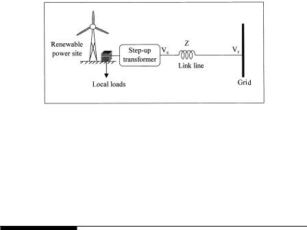
FIGURE 13-8

Equivalent circuit of renewable power plant connected to grid via transmission line link.

When the grid is disconnected for any reason, the generator will experience a loss of frequency regulation, as the frequency synchronizing signal derived from the grid lines is now lost. When a change in frequency is detected beyond a certain limit, the automatic control can shut down the system, cutting off all possible sources of excitation.

13.3 Operating Limit

The link line connecting the renewable power site with the utility grid introduces the operating limit in two ways, the voltage regulation and the stability limit. In most cases, the line can be considered as an electrically short transmission line. The ground capacitance and the ground leakage resistance are generally negligible and are ignored. The equivalent circuit of such a line, therefore, reduces to a series resistance R and reactance L (Figure 13-8). Such an approximation is valid in lines up to 50 miles long. The line carries power from the renewable site to the utility grid, or from the grid to the renewable site to meet local peak demand. There are two major effects of the transmission line impedance, one on the voltage regulation and the other on the maximum power transfer capability of the link line.

13.3.1Voltage Regulation

The phasor diagram of the voltage and current at the sending and receiving ends are shown in Figure 13-9. Since the shunt impedance is negligible, the sending end current Is is the same as the receiving end current Ir, i.e., Is = Ir = I. The voltage at the receiving end is the vector sum of the sending end voltage plus the impedance voltage drop I·Z in the line, i.e.:

© 1999 by CRC Press LLC

FIGURE 13-9

Phasor diagram of the link line carrying rated current.

The voltage regulation is defined as the rise in the receiving end voltage, expressed in percent of the full load voltage, when full load at a specified power factor is removed, holding the sending end voltage constant. That is as follows:

Vfl

where Vnl = magnitude of receiving end voltage at no load = Vs Vfl = magnitude of receiving end voltage at full load = Vr

With reference to the phasor diagram of Figure 13-9, Vnl = Vs and Vfl = Vr. The voltage regulation is a strong function of the load power factor. For the same load current at different power factors, the voltage drop in the line is the same, but is added to the sending end voltage at different phase angles to derive the receiving end voltage. For this reason, the voltage regulation is greater for lagging power factor, and the least or even negative for leading

power factor.

In Figure 13-9, suppose the magnitude of Vr and I are held constant and the power factor of the load is varied from zero lagging to zero leading. The vector Vs will vary such that its end point will lie on a semicircle since the magnitude I · (R + jX) is constant.1 Such a circle diagram is useful for plotting the sending end voltage versus load power factor for the given load voltage and KVA.

© 1999 by CRC Press LLC

If the voltages at both ends of the lines are held constant in magnitude, the receiving end real power and reactive power points plotted for several loads would lie on a circle known as the power circle diagram. The reader is referred to Stevenson1 for further reading on the transmission line circle diagrams.

13.3.2Stability Limit

The direction of the power flow depends on the sending and receiving end voltages, and the electrical phase angle between the two. However, the maximum power the line can transfer while maintaining stable operation has a limit. We derive below the stability limit assuming that the power flows from the renewable power site to the grid, although the same limit applies in the reverse direction as well. The series resistance in most lines is negligible, hence, is ignored here.

The power transferred to the grid by the transmission line is as follows:

Using the phasor diagram of Figure 13-9, the current I can be expressed as follows:

The real part of this current is as follows:

This, when multiplied with the receiving end voltage Vr, gives the following power:

Thus, the magnitude of the real power transferred by the line depends on the power angle δ. If δ > 0, the power flows from the site to the grid. On the other hand, if δ < 0, the site draws power from the grid.

The reactive power depends on (Vs–Vr). If Vs > Vr, the reactive power flows from the site to the grid. If Vs < Vr, the reactive power flows from the grid to the site.

© 1999 by CRC Press LLC

FIGURE 13-10

Power versus power angle showing static and dynamic stability limits of the link line.

Obviously, the power flow in either direction is maximum when δ = 90° (Figure 13-10). Beyond Pmax, the link line becomes unstable and will fall out of synchronous operation. That is, it will lose its ability to synchronously transfer power from the renewable power plant to the utility grid. This is referred to as the steady state stability limit. In practice, the line loading must be kept well below this limit to allow for transients such as sudden load steps and system faults. The maximum power the line can transfer without losing the stability even during system transients is referred to as the dynamic stability limit. In typical systems, the power angle must be kept below 10° to 20° to assure dynamic stability.

Since the generator and the link line are in series, the internal impedance of the generator is added in the line impedance for determining the maximum power transfer capability of the link line, the dynamic stability and the steady state performance.

13.4 Energy Storage and Load Scheduling

For large wind and pv plants on grid, it may be economical to store some energy locally in the battery or other energy storage systems. The short-term peak demand is met by the battery without drawing from the grid and paying the demand charge. For formulating the operating strategy for scheduling and optimization, the system constraints are first identified. The usual constraints are then battery size, the minimum on/off times and ramp rates for the thermal units, the battery charge and discharge rates, and the renewable capacity limits. The optimization problem is formulated to minimize

© 1999 by CRC Press LLC

TABLE 13-1

Production Cost of 300 MW Thermal-pv-Battery System

the cost of all thermal and renewable units combined subject to the constraints by arriving at the best short-term scheduling. This determines the hours for which the baseload thermal units of the electrical power company should be taken either off-line or on-line. The traditional thermal scheduling algorithms, augmented Lagrangian relaxation, branch and bound, successive dynamic programming or heuristic method (genetic algorithms and neural networks), can be used for minimizing the cost of operating the thermal units with a given renewable-battery system. Marwali et al.2 has recently utilized the successive dynamic programming to find the minimum cost trajectory for battery and the augmented Langrangian to find thermal unit commitment. In a case study of a 300 MW thermal-pv-battery power plant, the authors have arrived at the total production costs shown in Table 13-1, where the battery hybrid system saves $54,000 per day compared to the thermal only.

13.5 Utility Resource Planning Tool

The wind and photovoltaic power, in spite of their environmental, financial, and fuel diversity benefits, are not presently included in the utility resource planning analysis because of the lack of the familiarity and analytical tools for nondispatchable sources of power. The wind and pv powers are treated as nondispatchable for not being available on demand. The Massachusetts Institute of Technology’s Energy Laboratory has developed an analytical tool to analyze the impact of nondispatchable renewables on the New England’s power systems operation. Cardell and Connors3 have applied this tool for analyzing two hypothetical wind farms totaling 1,500 MW capacity for two sites, one in Maine and the other in Massachusetts. The average capacity factor at these two sites is estimated to be 0.25. This is good, although some sites in California have achieved the capacity factor of 0.33 or higher. The MIT study shows that the wind energy resource in New England is comparable to that in California. The second stage of their analysis developed the product cost model, demonstrating the emission and fuel cost risk mitigation benefits of the utility resource portfolios incorporating the wind power.

© 1999 by CRC Press LLC

References

1.Stevenson, W. D. 1962. “Elements of Power System Analysis,” New York, McGraw Hill Book Company, 1962.

2.Marwali, M. K. C., Halil, M., Shahidehpour, S. M., and Abdul-Rahman, K. H. 1997. “Short-term generation scheduling in photovoltaic-utility grid with battery storage,” IEEE paper No. PE-184-PWRS-16-09, 1997.

3.Cardell, J. B. and Connors, S. R. 1997. “Wind power in New England, modeling and analyses of nondispatchable renewable energy technologies,” IEEE Paper No. PE-888-PWRS-2-06, 1997.

© 1999 by CRC Press LLC

14

Electrical Performance

14.1 Voltage Current and Power Relations

The power systems worldwide are 60 Hz or 50 Hz AC three-phase systems. The three coils (phases) of the generator are connected in Y or ∆ as shown in Figure 14-1. In the balanced three-phase operation, the line-to-line voltage, the line current and the three phase power in terms of the phase voltage and current are given by the following equations, with notations marked in Figure 14-1.

In the Y connected system:

Where pf = power factor

In the ∆ connected system:

VL = Vph

P3−ph = 3 VL IL pf

For steady state or dynamic performance studies, the system components are modeled so as to represent the entire system. The power generator, the rectifier, the inverter, and the battery models were discussed in the earlier chapters. The components are accurately modeled to represent the conditions under which the performance is to be determined. This chapter concerns itself with the system level performance.

© 1999 by CRC Press LLC

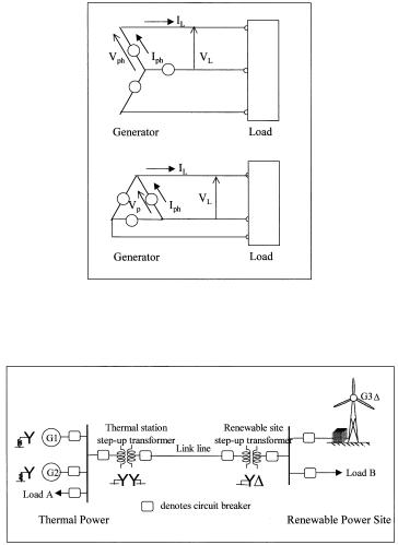
FIGURE 14-1

Three-phase AC systems is connected in Y or ∆.

FIGURE 14-2

One-line schematic diagram of grid-connected wind farm.

One-line diagram is widely used to represent the three phases of the system. Figure 14-2 is an example of a one-line diagram of the grid-connected system. On the left hand side are two Y-connected synchronous generators, one grounded through a reactor and one grounded through a resistor, supplying power to load A. On the right hand side is the wind power site with one ∆-connected induction generator, supplying power to load B, feeding the remaining power to the grid via the step up transformer, the circuit breakers, and the transmission line.

The balanced three-phase system is analyzed as the single-phase system. The neutral wire in the Y connection does not enter the analysis in any way, since it is at zero voltage and carries zero current.

© 1999 by CRC Press LLC

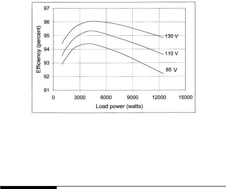
FIGURE 14-3

Power equipment efficiency varies with load with single maximum.

The unbalanced system, the balanced three-phase voltage on unbalanced load and faults need advanced analytical methods, such as the method symmetrical components.

14.2 Component Design for Maximum Efficiency

An important performance criterion of any system is the efficiency, measured as the power output as percentage of the power input. Since the system is as efficient as its components are, designing an efficient system means designing each component to operate at its maximum efficiency.

The electrical and electronic components while transferring power from the input side to the output side lose some power in the form of heat. In practical designs, the maximum efficiency of 90 to 98 percent is typical in large power equipment in hundreds of kW ratings, and 80 to 90 percent in small equipment in tens of kW ratings. The component efficiency, however, varies with load as shown in Figure 14-3. The efficiency increases with load up to a certain point beyond which it decreases. A good design maximizes the efficiency at the load that the equipment supplies most of the time. For example, if the equipment is loaded at 70 percent of its rated capacity most of the time, it is beneficial to have the maximum efficiency at 70 percent load. The method of achieving the maximum efficiency at a desired load level is presented below.

The total loss in any power equipment generally has two components. One remains fixed representing the quiescent no-load power consumption. The fixed loss primarily includes the eddy and hysteresis losses in the magnetic

© 1999 by CRC Press LLC

FIGURE 14-4

Loss components varying with load in typical power equipment.

parts. The other component varies with the current squared, representing the I2R loss in the conductors. For a constant voltage system, the conductor loss varies with the load power squared. The total loss is, therefore, expressed as (Figure 14-4) the following:

where P is the power delivered to the load (output), Lo is the fixed loss and k is the proportionality constant. The efficiency is given by the following:

For the efficiency to be maximum at a given load, its derivative with respect to the load power must be zero at that load. That is as follows:

This equation reduces to Lo = kP2. Therefore, the component efficiency is maximum at the load under which the fixed loss is equal to the variable loss. This is an important design rule, which can save significant electrical energy in large power systems.

© 1999 by CRC Press LLC

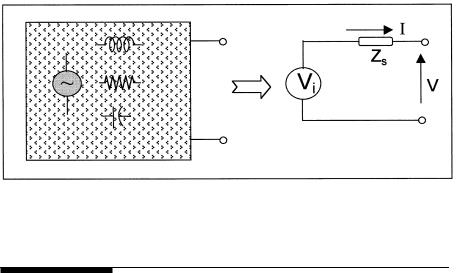
FIGURE 14-5

Thevenin’s equivalent circuit model of a complex power system.

14.3 Electrical System Model

The electrical network of any complexity can be reduced to a simple Thevenin’s equivalent circuit consisting of a single source voltage Vs and impedance Zs in series (Figure 14-5). The two parameters are determined as follows:

With the system operating at no load with all other parameters at rated values, the voltage at the open-circuit terminals equals the internal source voltage, since the internal voltage drop is zero. Therefore:

Vs = open-circuit voltage of the system.

For determining the source impedance, the terminals are shorted together and the terminal current is measured. Since the internal voltage is now consumed in driving the current through the only source impedance, then:

If Zs is to be determined by an actual test, the general practice is to short the terminals with the open-circuit voltage only several percentages of the rated voltage. The low level short-circuit current is measured and the full short-circuit current is calculated by scaling to the full-rated voltage. Any nonlinearality, if present, is accounted for.

The equivalent circuit is developed on a per phase basis and in percent or perunit bases. The source voltage, current, and the impedance are expressed in units of their respective base values at the terminal. The base values are defined as follows:

© 1999 by CRC Press LLC

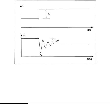
FIGURE 14-6

Transient response of the system voltage under sudden load step.

Vbase = Rated output voltage

Ibase = Rated output current, and

Zbase = Rated output voltage/Rated output current

14.4 Static Bus Impedance and Voltage Regulation

If the equivalent circuit model of Figure 14-5 is derived under the steady state static condition, the Zs is called the static bus impedance. The steady

state voltage rise on removal of the full load rated current is then ∆V = Ibase · Zs, and the voltage regulation is as follows:

Under a load step transient, partial or full, as in the case of a loss of load due to accidental opening of the load side breaker, the voltage oscillates until the transient settles to the new steady state value. If the load current rises in step as shown in Figure 14-6, the voltage goes through oscillation before settling down to a lower steady state value. The steady state change in the bus voltage is then given by the following:

∆V = ∆I · ZS

© 1999 by CRC Press LLC

FIGURE 14-7

Deadbands in the feedback voltage control system avoid the system flutter.

The feedback voltage control system responds to bring the bus voltage deviation back to the rated value. However, in order not to flutter the system more than necessary, the control system is designed with suitable deadbands. For example, Figure 14-7 shows a 120 voltage photovoltaic system with battery with two deadbands in its control system.

14.5 Dynamic Bus Impedance and Ripple

If the circuit model of Figure 14-5 is derived under the dynamic condition, that is for an incremental load, the source impedance is called the dynamic bus impedance, and is denoted by Zd. It can be either calculated or measured as follows. With the bus in operational mode supplying the rated load, inject a small high frequency AC current Ih into the bus using an independent grounded current source (Figure 14-8). The high frequency voltage perturbation in the bus voltage is measured and denoted by Vh. The dynamic bus impedance at that frequency is then:

V

Zd = I h (14-8)

h

The ripple is the term used to describe periodic glitches in the current or the voltage, generally of high frequency. Ripples are commonly found in systems with power electronics components, such as rectifiers, inverters, battery chargers, or other switching circuits. The ripples are caused by the

© 1999 by CRC Press LLC

FIGURE 14-8

Harmonic and dynamic source impedance test measurement set-up.

transistors switching on and off. The ripple frequencies are integer multiples of the switching frequency. The ripples are periodic but not sinewave and are superimposed on the fundamental wave.

The ripple voltage induced on the bus due to ripple current is given by the following:

The ripple is minimized by the capacitor connected to the bus or preferably at the load terminals of the component causing ripples. The ripple current is then supplied or absorbed by the capacitor, rather than by the bus, thus, improving the quality of power.

14.6 Harmonics

The harmonics is the term used to describe the higher frequency sinewave currents or voltages superimposed on the fundamental sinewave. Phasecontrolled power switching is one source of harmonics. The harmonics are also generated by magnetic saturation in power equipment. With no saturation present in the magnetic circuit, the generator and the transformer behave linearly, but not so with saturation. The saturated magnetic circuit requires non-sinewave magnetizing current.

The usual method of analyzing the system with harmonics is to determine the performance of the system for each harmonics separately and then to superimpose the results. The system is represented by the equivalent circuit for each harmonic.

The fundamental equivalent circuit of the electrical generator is represented by the d-axis and q-axis.1-2 In the nth harmonic equivalent circuit, the

© 1999 by CRC Press LLC

harmonic inductance Ln , being for high frequency, is the average of the subtransient inductance in the d and q axes, that is as follows:

and the reactance for the harmonic of order n is given by the following:

where fn = nth harmonic frequency f = fundamental frequency.

In single-phase or three-phase AC currents having positive and negative portions of the cycle symmetrical, the odd number of harmonics are absent. That is, In = 0 for n = 2, 4, 6, 8, and so on. In three-phase load circuits fed by transformers having the primary windings connected in delta, all triple harmonics are absent in the line currents, that is In = 0 for n = 3, 9, 15, and so on.

In the inverter circuit having m-pulse full bridge circuit, the harmonics present are of the order n = mk ± 1, where k = 1, 2, 3, 4, and so on. For example, the harmonics present in a 6-pulse inverter are 5, 7, 11, 13, 17, 19. On the other hand, the harmonics present in 12-pulse inverter are 11, 13, 23, 25. The magnitude and phase of the harmonic currents are found to be inversely proportional to the harmonic order n, that is as follows:

where I1 is the fundamental current. This formula gives approximate harmonic contents in 6 and 12-pulse inverters as given in the first two columns of Table 14-1, which clearly shows the benefits of using 12-pulse converters.

TABLE 14-1

Harmonic Contents of the 6-pulse and 12-pulse Converters

© 1999 by CRC Press LLC

The actually measured harmonic currents are lower than those given by the approximate Equation 14-12. The IEEE Standard-519 gives the current harmonic spectrum in typical 6-pulse converters as listed in the last column of Table 14-1.

The harmonic currents induce harmonic voltage on the bus. The harmonic voltage of order n is given by Vn = In · Zn , where Zn is the nth harmonic impedance. The harmonic impedance can be derived in a manner similar to the dynamic impedance, in that a harmonic current Ih is injected to or drawn from the bus and the resulting harmonic voltage Vn is measured. In a rectifier circuit drawing harmonic currents In provides a simple circuit which works as the harmonic current load. If all harmonic currents are measured, then the harmonic impedance of order n is given by the following:

Zn = VnIn , where n = mk ± 1, and k = 1, 2, 3, and so on. (14-13)

14.7 Quality of Power

The requirement of the quality of power at the grid interface is a part of the power purchase contracts between the utility and the renewable power plant. The rectifier and inverter are the main components contributing to the power quality concerns. The grid-connected power systems, therefore, need converters which are designed to produce high quality, low distortion AC power acceptable for purchase by the utility company. The power quality concerns become more pronounced when the renewable power system is connected to small capacity grids using long low voltage link.

Until recently, there was no generally acceptable definition of the quality of power. However, the International Electrotechnical Commission and the North American Reliability Council have developed working definitions, measurements and design standards.

Broadly, the power quality has three major components for measurements:

•the total harmonic distortion generated by the power electronic equipment, such as rectifier and inverter.

•the transient voltage sags caused by system disturbances and faults.

•periodic voltage flickers.

14.7.1Harmonic Distortion

Any non-sinusoidal alternating voltage V(t) can be decomposed in the following Fourier series:

© 1999 by CRC Press LLC

The first component on the right hand side of the above equation is the fundamental component, whereas all other higher frequency terms (n = 2,3…∞) are the harmonics.

The Total Harmonic Distortion Factor is defined as follows:

The THD is useful in comparing the quality of AC power at various locations of the same power system, or of two or more power systems. In a pure sine wave AC source, THD = 0. The greater the value of THD, the more distorted the sinewave, resulting in more I2R loss for the same useful power delivered. This way the quality of power and the efficiency are related.

As seen earlier, the harmonic distortion on the bus voltage caused by harmonic current In drawn by any nonlinear load is given by Vn = In Zn. It is this distortion in the bus voltage that causes the harmonic current to flow even in pure linear resistive load, called the victim load. If the renewable power plant is relatively small, the nonlinear electronic loads may cause significant distortion on the bus voltage, which then supplies distorted current to the linear loads. The harmonics must be filtered out before feeding power to the grid. For a grid interface, having the THD less than 3 percent is generally acceptable. The IEEE Standard-519 limits the THD for the utility grade power to less than 5 percent.

It can be seen that harmonics do not contribute to delivering useful power, but produce I2R heating. Such heating in generators, motors, and transformers is more difficult to dissipate due to their confined designs, as opposed to open conductors. The 1996 National Electrical Code® requires all distribution transformers to state their k-ratings on the permanent nameplate. This is useful in sizing the transformer for use in a system having a large THD. The k-rated transformer does not eliminate line harmonics. The k-rat- ing merely represents the transformer’s ability to tolerate the distortion. The unity k rating means the transformer can handle the rated load drawing pure sinewave current. The transformer supplying only electronic load may require high k-rating of 15 to 20.

A recent study funded by the Electrical Power Research Institute reports the impact of two pv solar parks on the power quality of the grid-connected distribution system3. The harmonic current and voltage waveforms were monitored under connection/disconnection tests over a nine month period ending March 1996. The current injected by the pv park had a total distortion below the 12 percent limit set by the IEEE-519-1992 standard. However, even the individual harmonic components between 18 and 48, except the 34th, exceeded the IEEE-519 standard. The total voltage distortion, however, was minimal.

A rough measure of quality of power is the ratio of the peak to rms voltage measured by the true rms voltmeter. In a pure sine wave, this ratio is 2 = 1.414. Most acceptable bus voltages will have this ratio in the 1.3 to 1.5 range,

© 1999 by CRC Press LLC

FIGURE 14-9

Allowable voltage deviation in utility-grade power versus time duration of the deviation. (Adapted from the American National Standards Institute.)

which can be used as a quick approximate check on the quality of power at any location in the system.

14.7.2Voltage Transients and Sags

The bus voltage can deviate from the nominally-rated value due to many reasons. The deviation that can be tolerated depends on its magnitude and the time duration. Small deviations can be tolerated for a longer time than large deviations. The tolerance band is generally defined by voltage versus time (v-t) limits. Computers and business equipment using microelectronic circuits are more susceptible to the voltage transients than the rugged power equipment such as motors and transformers. The power industry has developed an array of protective equipment. Even then, some standard of power quality must be maintained at the system level. For example, the system voltage must be maintained within the v-t envelope shown in Figure 14-9, where the solid line is that specified by the American National Standard Institute (ANSI). The right hand side of the band comes primarily from the steady state performance limitations of motors and transformer-like loads, the middle portion comes from visible lighting flicker annoyance considerations, and the left hand side of the band comes from the electronic load susceptibility considerations. The left hand side curve allows larger deviations in the microsecond range based on the volt-second capability of the power supply magnetics. The ANSI requires the steady state voltage of the utility source to be within 5 percent, and short-time frequency deviations less than 0.1 Hz.

© 1999 by CRC Press LLC

FIGURE 14-10

Thevenin’s equivalent circuit model of induction generator for voltage flicker study.

14.7.3Voltage Flickers

The turbine speed fluctuation under fluctuating wind, causes slow voltage flickers and current variations that are large enough to be detected as flickers in fluorescent lights. The relation between the fluctuation of mechanical power, the rotor speed, the voltage, and the current is analyzed by using the dynamic d and q-axis model of the induction generator or the Thevenin’s equivalent circuit model shown in Figure 14-10. If we let:

R1, R2 = resistance of stator and rotor conductors, receptively.

x1, x2 = leakage reactance of stator and rotor windings, receptively. xm = the magnetizing reactance.

x = the open-circuit reactance.

x’= the transient reactance.

τo = the rotor open-circuit time constant = (x2+xm)/(2πfR2). s = the rotor slip.

f = frequency.

ET = the machine voltage behind the transient reactance. V = the terminal voltage.

Is = the stator current.

then, the value of ET is obtained by integrating the following equation:

And the stator current is as follows:

© 1999 by CRC Press LLC

The mechanical equation, taking into account the rotor inertia, is as follows:

where Pe = electrical power delivered by the generator Pm = mechanical power of the wind turbine

H = rotor inertia constant in seconds = 1/2 J ω2/Prated J = moment of inertia of the rotor, and

ω = 2 π f

The electrical power is the real part of the product of the ET and Is*:

where Is* is the complex conjugate of the stator current.

The mechanical power fluctuations can be expressed by a sinewave superimposed on the steady value of Pmo:

where ω1 = rotor speed fluctuation corresponding to the wind power fluctuation.

Solving these equations by iterative process on the computer, Feijoo and Cidras4 showed that fluctuations of a few hertz can cause noticeable voltage and current fluctuations. Several hertz fluctuations are too small to be detected at the machine terminals. The high frequency fluctuations, in effect, are filtered out by the wind turbine inertia, which is usually large. That leaves only a band of the fluctuations that could be detected at the generator terminals.

The flickers caused by the wind fluctuations may be of a concern in low voltage transmission lines connecting to the grid. The voltage drop related to the power swing is small in high voltage lines because of small current fluctuation for a given wind fluctuation.

14.8 Renewable Capacity Limit

A recent survey made by Gardner5 and Risø National Laboratory6 in the European renewable power industry indicates that the grid interface issue is one of the economic factors limiting full exploitation of the available wind resources. The regions of high wind power potentials have weak existing electrical grids. In many developing countries such as India, China, and

© 1999 by CRC Press LLC

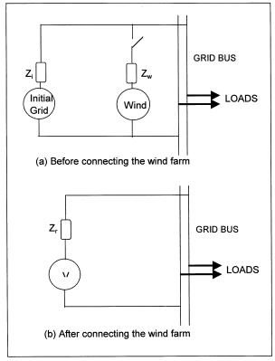
FIGURE 14-11

Thevenin’s equivalent circuit model of the grid and wind farm for evaluation of the grid interface performance for evaluating the system stiffness at the interface.

Mexico, engineers are faced with locating sites that are also compatible for interfacing with the grid from the power-quality point of view. The basic consideration in such decisions is the source impedance before and after making the connection. Another way of looking at this issue is the available short-circuit MVA at the point of the proposed interconnection, also known as the system stiffness or the fault level.

14.8.1System Stiffness

One way of evaluating the system stiffness after making the interconnection is by using the Thevenin’s equivalent circuit of the grid and the renewable plant separately as shown in Figure 14-11.

If we let:

V = network voltage at the point of the proposed interconnection.

Zi = source impedance of the initial grid before the interconnection.

© 1999 by CRC Press LLC

Zw = source impedance of the wind farm.

Zl = impedance of the interconnecting line from the wind farm to the grid.

then, after connecting the proposed wind capacity with the grid, the combined equivalent Thevenin’s network would be as shown in (b), where:

where Zt = total combined source impedance of the two systems.

The combined short circuit MVA at the point of the interconnection is then:

The higher the short-circuit MVA, the stiffer the network. Certain minimum grid stiffness in relation to the renewable power capacity is required to maintain the power quality of the resulting network. This consideration limits the total wind capacity that can be added at a site under consideration. The wind capacity exceeding that limit may be a difficult proposal to sell to the company in charge of the grid.

Not only the magnitude of Zt is important, the resistance R and the reactance X components of Zt have their individual importance. The fundamental circuit theory dictates that the real and reactive power in any electrical network must be separately maintained in balance. Therefore, the real and reactive components of the wind generator impedance would impact the network, more so in a weaker grid. The R/X ratio is often found to be 0.5, which is generally satisfactory for fixed-speed wind generators. Lower R/X ratio may pose another limitation on designing the system.

The fault current decays exponentially as e–R/X. Low R/X ratio causes the fault currents to linger on, making the fault protection relaying more difficult. The voltage regulation (variation from zero to full load on the wind farm) is yet another design consideration that is impacted by the R/X ratio. The estimated voltage regulation of the wind farm must be compared with the contractual limit with the utility. In doing so, the actual continuous maximum load the wind farm can deliver must be taken into account, not the nominal rating which can be much higher. The acceptable voltage regulation in industrial countries is typically 5 percent, and 7 percent in developing countries.

Starting the wind turbine as the induction motor causes an inrush of current from the grid, causing a sudden voltage drop for a few seconds. This can be intolerable by the grid line. Most countries limit this transient voltage dip to 2 to 5 percent, the higher value prevailing in the developing countries.

© 1999 by CRC Press LLC

TABLE 14-2

Acceptable Voltage Variation at

Distribution Points (Low Voltage

Consumers May See Wider Variations)

TABLE 14-3

Allowable Step-Change in Voltages a Customer can Cause by Step Loading or Unloading

TABLE 14-4

Renewable Power Generation Limit

in Percent of the Grid Short Circuit

Capacity at the Point of Interface

The acceptable voltage variations in the grid voltage at the distribution point in four countries are given in Table 14-2. The limit on the step-change a customer can cause on loading or unloading is listed in Table 14-3. It is complex to determine the maximum renewable capacity that can be allowed at a given site which will meet all these complex requirements. It may be even more difficult to demonstrate the compliance. Under the situation, some countries impose limits in percent of the grid short-circuit capacity. For example, such limits in Germany and Spain are listed in Table 14-4, but similar limits are evolving in other countries.

The power quality standards applicable specifically to grid-connected wind farms are being drafted by the International Electrotechnical Commission. It is expected that such standards would be more realistic than the rigid criteria based on the ratio of the wind turbine capacity to the short-circuit MVA of the grid. The ultimate results would be consistent and predictable

© 1999 by CRC Press LLC

FIGURE 4-12

Thunderstorm frequency in the United States and Southern Canada. The contour lines indicate the average number of days per year with thunderstorm occurrence.

understanding on the power quality requirements and less cost-related in designing wind farms to comply with the power quality issues.

Again, in order to control the quality of power, a rough rule of thumb has been to keep the renewable power plant capacity in MW less than the grid line voltage in kV if the grid is stiff (large). On a weak grid, however, only 10 or 20 percent of this capacity may be allowed.

14.9 Lightning Protection

The risk of mechanical and thermal damage to the blades and the electrical systems due to lightning is minimized by a coordinated protection scheme using lightning arresters and spark gaps6-7 in accordance with the International Standards. The IEC Standard -1024-1 covers the requirements for protection of structures against lightning. The electrical generator and transformers are designed with certain minimum Basic Insulation Level (BIL) consistent with the lightning risk in the area. The risk is proportional to the number of thunderstorms per year in the area. Figure 14-12 depicts the number of thunderstorms per year in the United States and southern Canada.

Tall towers are more vulnerable to the lightning risk. Among the valuable new experience in the wind power industry is that the offshore wind power towers experience a higher than average incidence of lightning strikes. Based on such experience, the system manufacturer has addressed the design problems. Figure 14-13 is one such solution developed by Vestas Wind Systems of Denmark. The lightning current is dispersed to the ground though a series of spark gaps and equipotential bonding at joints. The transformer is protected by placing it inside the tower.

© 1999 by CRC Press LLC

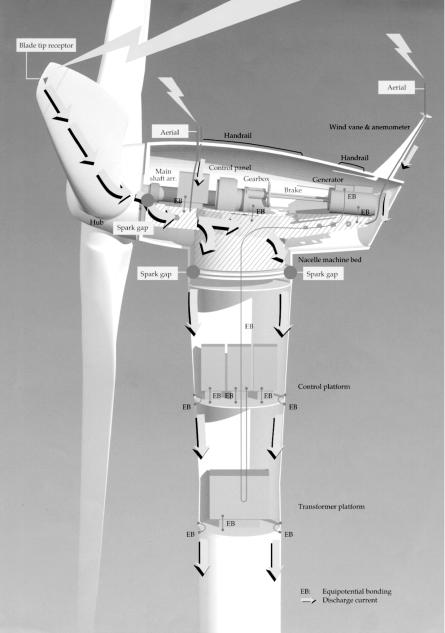
FIGURE 14-13

Lightning protection of the wind tower. (Source: Nordtank Energy Group/NEG Micon, Denmark. With permission.)

© 1999 by CRC Press LLC

14.10National Electrical Code® on Renewable Power Systems

The 1996 revision of the National Electrical Code8 has established electrical system requirements on the wind and photovoltaic power systems. The photovoltaics are covered in Article 690. The Article 705 covers all renewable and cogeneration power systems, including the wind, which is reproduced in Appendix 1 of this book.

References

1.Adkins, B. 1964. “The General Theory of Electrical Machines,” London, Chapman and Hall, 1964.

2.Kron, G. 1967. “Equivalent Circuits of Electrical Machines,” New York, Dover Publications, 1967.

3.Oliva, A. R., Balda, J. C., McNabb, D. W., and Richardson, R. D. 1997. “Power quality monitoring of a pv generator,” IEEE paper No. PE-507-EC0-07, 1997.

4.Feijoo, A and Cidras, J. 1997. “Analyses of mechanical power fluctuations in asynchronous WECs,” IEEE paper No. PE-030-EC-0-1 0, 1997.

5.Gardner, P. 1997. “Wind farms and weak networks,” Wind Directions, Magazine of the European Wind Energy Association, London, July 1997.

6.Risø National Laboratory. 1996. “Power quality and grid connection of wind turbines” — Summary report R-853, Denmark, October 1996.

7.Lewis, W. W. 1965. “The Protection of Transmission Systems Against Lightning,” New York, Dover Publications, 1965.

8.National Fire Protection Association. 1996. National Electrical Code Handbook, 7th Ed., Quincy, MA, 1996.

© 1999 by CRC Press LLC

15

Plant Economy

The economic viability of a proposed plant is influenced by several factors that contribute to the expected profitability. Since the profitability inadvertently varies with variations in the contributing factors, the sensitivity of the expected profitability is analyzed with variances around their expected values. The sensitivity analysis raises the confidence level of potential investors. This is important for both the wind and pv systems, but more so for wind systems whose profitability is extremely sensitive to the wind speed variations.

The primary factors contributing to the economic viability of the plants are discussed in this chapter. The results are displayed in easy-to-use charts for screening the profitability of a proposed plant.

15.1 Energy Delivery Factor

The key economic performance measure of a power plant is the electrical energy it delivers over the year. Not all power produced is delivered to the paying customers. A fraction of it is used internally to power the control equipment, meeting the power equipment losses and for the housekeeping functions such as lighting. In a typical wind farm or pv park, about 90 percent of the power produced is delivered to the customers, and the remaining is self-consumed for the plant operation.

The quantity of energy delivered depends on the peak power capacity of the site and how fully that capacity is utilized over every hour of the year. The normalized measure of the power plant performance is the Energy Delivery Factor (EDF). It is defined as the ratio of the electrical energy delivered to the customers to the energy that can be delivered by the plant if it could be operated at the fully installed capacity during all 8,760 hours of the year, that is as follows:

Installed capacity Number of hours in the year

© 1999 by CRC Press LLC

Since the load power varies over the time, the EDF takes the integral form:

year

∫ Po dt

where Pm = Plant capacity (the maximum power the plant can deliver) Po = Power delivered to the customers at any time t

The EDF is usually determined by bookkeeping the sum of the energy delivered over a continuous series of small discrete time intervals, that is as follows:

where Pavg = average power delivered over the small time interval ∆t.

The EDF is a figure of merit that measures how hard the plant is utilized to deliver the maximum possible energy. Not only does it include the energy conversion efficiencies of various components, it also accounts for the reliability, maintainability, and availability of the overall plant over the entire year.

The EDF is useful in comparing the economic utilization of one site over the other, or the annual performance of a given site. Wind plants operate with the annual average EDF around 30 percent, with some plants reporting EDF as high as 40 percent. This compares with 40 to 80 percent for the conventional plants. The base load plants operate at the higher end of the range.

The wind farm energy delivery factor varies with season and that must be taken into account. For example, the quarterly average EDF in England and Wales from the beginning of 1992 to the end of 1996 are shown in Figure 15-1. The operating data show rather wide variations, ranging from 15 to 45 percent. The EDF is high in the first quarter and low in the last quarter of every year. Even with the same kWh produced per year, the average price per kWh the plant may fetch could be lower if the seasonal variations are wide.

15.2 Initial Capital Cost

The capital cost depends on the size, site and the technology of the plant. Typical ranges for various types of large power plants are given in Table 15-1.

© 1999 by CRC Press LLC

FIGURE 15-1

Capacity factors of operating wind farms in England and Wales. (Source: U.K. Department of Trade and Industry, Renewable Energy Technology Status Report, August 1997. With permission.)

TABLE 15-1

Capital Cost for Various Power Technologies

The costs of technologically matured coal and gas turbine plants are rising with inflation, whereas the wind and pv plant costs are falling with new developments coming in the market. Therefore, the renewable power plant cost must be estimated with their component costs current at the time of procurement, which may be lower than those at the time of planning.

The percent breakdown of the component costs in the total initial capital cost of a typical wind farm is shown in Table 15-2. The single largest cost item is the turbine blades and rotor assembly, as expected.

15.3 Availability and Maintenance

The failure rates and effects determine the maintenance cost and availability of the plant to produce power. The past data on the operating experience is

© 1999 by CRC Press LLC

TABLE 15-2

Wind Power System Component Cost Contribution in Total

Capital Cost

(Land cost is not included)

used for learning lessons and making improvements. In the wind power industry, the failures, their causes and effects are recorded and periodically published by ISET, the solar energy research unit of the University of Kassel in Germany. Figure 15-2 summarizes the ISET database.2 The statistics show that 67 percent of the time during the reported failure period, the plant is nonoperational. Among the repairs needed to bring the plant back in operation, 20 percent are in the electrical power equipment and 19 percent are in the electronic controls. The major causes of the failure have been 28 percent in the control systems and 24 percent in the component defects. The failure rates are declining from this level with the design improvements made since then.

The overall availability of the plant is defined as the ratio of hours the plant is operating to deliver full power over the total hours in the year. It is impacted by downtimes due to repairs and routine maintenance. Significant improvements in reliability and maintainability have pushed the availability of modern renewable power plants up to 95 percent in recent years. The availability factor, however, is reflected in the energy delivery factor EDF.

15.4 Energy Cost Estimates

The principal decision-making parameter of an electrical power plant is the unit cost of energy (UCE) per kWh delivered to the paying consumers. It takes into account all economy factors discussed above, and is given by the following:

© 1999 by CRC Press LLC

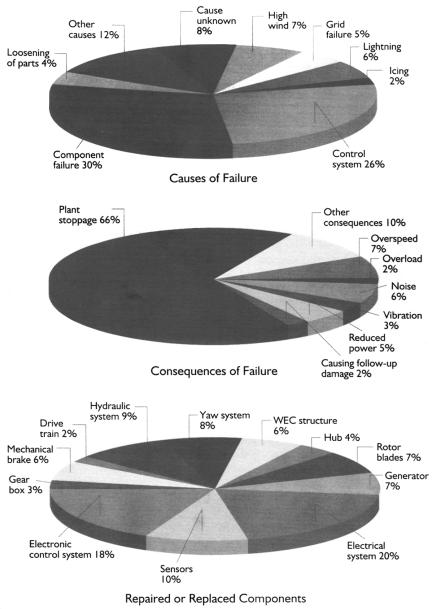
FIGURE 15-2

Wind power plant failure, cause, effect, and repair statistics. (Source: Institute of Solar Energy and Technology, University of Kassel, Germany, With permission.)

where ICC = Initial capital cost, including land cost and startup cost up to the time the first unit of energy is sold

AMR = Amortization rate per year as a fraction of the ICC

© 1999 by CRC Press LLC

The amortization rate AMR reflects the cost of money, generally taken as 0.10 to 0.20 depending on the prevailing mortgage interest rates available for such a project. The energy delivery factor EDF accounts for the variations in the impinging energy (sun intensity or wind speed) at the proposed site, and all downtimes, full or partial. It is also a strong function of the reliability and maintainability of the plant over the entire year.

The present costs of various energy sources are summarized in Table 15-3. It shows that the wind power now compares well with the conventional coal thermal power.

15.5 Sensitivity Analysis

Accurately estimating the cost of electricity produced is not sufficient. The project planners must also carry out the sensitivity analysis, in that the energy cost is estimated with a series of input parameters deviating on both sides of the expected values. The sensitivity of the energy cost on the following two factors is discussed in this section:

•variation in the wind speed.

•variation in solar irradiation.

15.5.1Effect of Wind Speed Variations

Since the energy output of the wind plant varies with the cube of the wind speed, a several percent change in the speed can have significant impact on

TABLE 15-3

Energy Generation Cost with Various

Power Technologies

© 1999 by CRC Press LLC

FIGURE 15-3

Sensitivity analysis of wind electricity cost with variation in wind speed around the expected annual mean of 10 meter/second.

the plant economy. For example, if the annual average wind speed is 10 m/s, the unit cost of energy is calculated for wind speeds ranging from 8 to 12 m/s. The plant site is considered economically viable only if the plant can be profitable at the low end of the probable range. Figure 15-3 illustrates the result of a sensitivity study. It shows that the cost of electricity can be as low as one-half or as high as twice the expected value if the wind speed turns out to be 2 m/s higher or lower than the expected value of 8 m/s.

15.5.2Effect of Tower Height

Tower height varies from approximately four rotor diameters for turbines in a few kW ratings to little over one diameter for turbines in several hundred kW ratings. The tower height for large turbines is primarily determined by the tower structure and the foundation design considerations. The tower height of small turbines is determined from the wind speed at the hub. The higher the hub, the higher the wind speed.

As seen in Table 15-2 earlier, the turbine cost constitutes 25 percent of the total wind farm cost. Since the wind speed increases with tower height, we can produce more energy from the same turbine by installing it on a taller tower, thus reducing the cost of energy produced.

We define E1 as contribution of the turbine cost in the total energy cost per square meter of rotor swept area. The E1 is therefore measured in $/kWh·m2. Since power is proportional to the rotor diameter squared and the wind speed cubed, we write the following:

© 1999 by CRC Press LLC

The energy captured over the life of the turbine is also proportional to the same parameters, i.e., D2 and V3. In a matured competitive market, the rotor cost would be proportional to the swept area, hence D2, although it is far from that stage in the current rapidly evolving market. However, assuming the competitive market E1 is as follows:

As seen earlier in Equation 4-34, the wind speed varies with tower height in the exponential relation:

where H = tower height at the hub.

Combining Equations 15-6 and 15-7, we obtain:

The parameter α varies with the terrain type. Table 4-3 in Chapter 4 gives this parameter value of 0.10 over the ocean, 0.40 over urban areas with tall buildings and the often used average of 0.15 (~1/7) in areas with foot high grass on flat ground. Even higher value of 0.43 was estimated for a New England site at Stratton, Mt. Vermont.1 With such variations in α, the wind speed can vary with H over a wide range from H0.3 to H1.3.

Equation 15-8 clearly indicates that the turbine contribution in cost of energy per unit swept area decreases at least with the square root of the tower height. With the average value of α of 1/7, the turbine cost contribution is approximately:

In rough terrain, the tower height can be extremely beneficial as shown by the following equation with α = 0.4:

Equations 15-9 and 15-10 indicate that there is not much benefit in increasing the tower height of the offshore installations. However, on rough terrain, increasing the tower height from 30 to 60 meters would decrease the contribution of the turbine cost per kWh/m2 by 56 percent, a significant reduction.

© 1999 by CRC Press LLC

•expected economic life of the plant.

•operating and maintenance cost.

•average selling price of the energy generated from the farm.

A detailed multivariable profitability analysis with the above parameters is always required before making financial investments. Potential investors can make initial profitability assessment using screening charts. The following sections present easy-to-use profitability charts for initial screening of the wind and pv power plant sites.

15.6.1Wind Farm Screening Chart

Figure 15-4 is a wind farm profitability screening chart based on cost of capital (discount rate) of 8 percent, project life of 15 years, initial cost of 1,100 European currency units per kW capacity, and the operating and maintenance cost of 3 percent of the initial project cost.3 The chart takes into account the inflation at a constant rate, i.e., the costs and revenues rising at the same rate. The taxes on sales, if any, must be deducted from the average selling price before it is entered in reading the chart. An example for using the chart follows:

At a site with 7.5 m/s wind speed at hub height, the profitability index would be zero (a break-even point) if the energy can be sold at 0.069 ECU/kWh. If the energy price is 0.085 ECU/kWh, the profitability index would be 0.30, generally an attractive value for private investors. At a site with only 7 m/s wind speed, the same profitability can be achieved if the energy can be sold at 0.097 ECU/kWh.

15.6.2pv Park Screening Chart

Similar screening charts for pv stand-alone or grid-connected systems are shown in Figures 15-6 and 15-7.4 For these charts, the yearly energy delivery Ey in kWh/year is defined as the following:

where Kp = performance ratio of the system

Hy = yearly solar irradiation in the plane of the modules, kWh/m2/year Ppk = installed peak power under the standard test conditions of 1 kW/m2 solar irradiation, the cell junction operating tempera-

ture of 25°C and the air mass of 1.5.

The pv energy conversion efficiency of the modules is included in Ppk. The typical values of Kp for well designed systems are 0.7 to 0.8 for gird-connected

© 1999 by CRC Press LLC

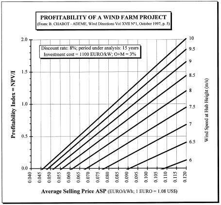
FIGURE 15-4

Profitability chart for wind farms. (Source: B. Chabot – ADME, France, and Wind Directions, Magazine of the European Wind Energy Association, London, October 1997. With permission.)

systems without batteries and delivering AC power using inverters, and 0.5 to 0.6 for stand-alone systems using batteries and delivering DC power.

The input to the figures are the initial capital cost of the pv system in dollars per peak watt capacity Iup, the cost of capital, the life of the plant, the operating and maintenance cost Kom , the yearly solar irradiation Hy, and the performance parameter Kp as defined above. With these inputs, the chart gives the overall discounted cost (ODC) of electricity delivered. The life of the plant in years, n, can be the desired payback period to recover the initial investment, or the full economic life of the plant. In the latter case, the ODC is known as the life cycle cost (LCC) of the energy delivered. The chart is prepared with typical values for large pv farms, such as Kp of 0.75, 8 percent cost of capital, 20 years life and 2 percent operating and maintenance cost.

© 1999 by CRC Press LLC

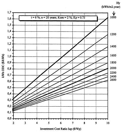
FIGURE 15-5

Overall discounted cost of pv energy. (Source: B. Chabot – ADME, France and Progress in Photovoltaic Research and Applications, Volume 6, p. 58, 1998. John Wiley & Sons Limited, Bristol, U.K.. With permission.)

An example of using Figure 15-5 follows. At a solar site with Hy of 2,000 kWh/m2/yr and the capital cost of 5 $/Wp, we see that the energy cost would be $0.40 per kWh delivered. For the cost of energy delivered to be below 0.20 $/kWh, the capital cost of the plant must be $2.50 per Wp. With new pv technologies being developed and made commercially available at lower costs, the capital cost below 3 $/Wp is realizable.

Being costlier than the wind power systems, the pv systems at present are more likely to be installed in remote areas where higher cost can be justified and partially offset by low interest loans. Figure 15-6 is cast in terms of the profitability index defined earlier. The parameters for this chart are the capital cost of 4 $/Wp, 3 percent cost of capital, 30 years economic life, 1 percent operating and maintenance cost and the performance parameter

© 1999 by CRC Press LLC

FIGURE 15-6

Profitability chart for photovoltaic power. (Source: B. Chabot – ADME, France and Progress in Photovoltaic Research and Applications, Volume 6, p. 62, 1998. John Wiley & Sons Limited, Bristol, U.K.. With permission.)

of 0.75 percent. For a solar irradiation of 2,000 kWh/m2/year and an average selling price of 20 cents/kWh, the profitability index would be 0.25, a reasonable number for private investors.

15.6.3Stand-Alone pv Versus Grid Line

In remote areas, where the grid power is not available and the wind is not an option, the customer who wants electricity has two options:

•pay the utility company for extending the line.

•install a pv power system at the site.

© 1999 by CRC Press LLC

FIGURE 15-7

Stand-alone pv plant or line extension costs for various levels of energy need based on average 1997 costs of Idaho Power Company.

The cost of extending the line may be prohibitive if the stretch is long. For a given distance of the line extension, the line cost is fixed. The economy of the electrical energy, therefore, clearly depends on the energy demand in kWh per day. Figure 15-7 is a screening chart for making economic choice between the line extension and a pv plant at site. It is developed using the 1997 average utility charges for line extension and pv modules price. As an example of using the chart, if the customer needs 10 kWh/day and lives three miles away from the nearest power line, the stand-alone pv at the site would be economical. If the distance were one mile instead, the line extension would be economical. The break-even distance for this customer is about 1.7 miles. For another customer who needs 20 kWh/day, the break-even distance is three miles.

In getting the line extension, rural utilities and their customers face conflicting interest. The utility is interested in controlling the cost, and the customer is interested in reliable power. In selected low population density areas of the U.S.A., some utility companies offer their customers a choice of installing a pv system as an alternative to costly emergency service and long stretches of the line dedicated to serve one or a few customers.

This is how some U.S. utility companies in rural areas are responding to potential pv customers:

•customer interested in electric power contacts the utility company.

•determination is made whether the point-of-service will be economically served by extending a line or by installing a pv system at the site.

•utility company develops the pv design.

•the system is installed by an independent contractor.

© 1999 by CRC Press LLC

•the total capital cost is paid by the utility company.

•the utility company is responsible for maintenance of the system.

•customer is billed a fixed monthly rate, rather than the amount based on the energy consumed.

This approach spreads out the burden of the initial capital cost on the customer.

15.7 Hybrid Economics

A detailed analytical tool to evaluate the economics of hybrid systems has been developed by the National Renewable Energy Laboratory. The newer version, Hybrid25 allows the user to determine basic economic figures for a particular simulation run. The economics module uses information from the performance simulation run and economic data supplied by the user. It computes parameters as the payback period, internal rate of return, cash flow, and equipment replacement expenses. The user has a wide versatility in determining the expense of the project and what inputs to include. Parameters such as grid extension, importation tariffs, systems administration costs, and taxes can be included in the analysis. The user may conduct comparisons between differing hybrid possibilities and power solutions, and determine approximate costs. Figure 15-8 is the computer screen displaying the choices available to the user. As indicated by the menu buttons, it includes wind, pv, diesel, and battery.

Hybrid2 allows user to conduct parametric analyses on certain cost parameters, such as fuel cost, discount rate, and inflation rate to help determine how the value of certain parameters can affect the viability of the project.

As for the project funding, there have been strong financial incentives for the renewable power in many countries around the world. However, the incentives have been declining because the renewables are becoming economically competitive on their own merits. More projects are being funded strictly on the commercial basis. Enviro Tech Investment Funds in the U.S.A. is a venture-capital fund supported by Edison Electric Institute (an association of investor-owned electric utility companies providing 75 percent of the nation’s electricity). The World Bank now includes the wind and pv in its landing portfolios. The first such loan was made to India in 1993. Several units in the World Bank group are jointly developing stand-alone projects in developing countries.

© 1999 by CRC Press LLC

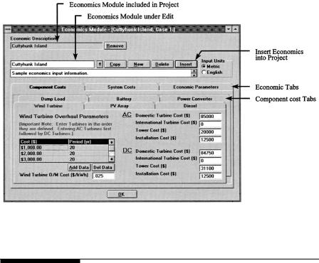
FIGURE 15-8

Hybrid2 economic simulation model. (Source: Ian Baring-Gould, National Renewable Energy Laboratory, Golden, Colorado. With permission.)

References

1.Cardell, J. B. and Connors, S. R. 1997. “Wind power in New England, modeling and analyses of nondispatchable renewable energy technologies,” IEEE Paper No. Power Engineering-888-PWRS-2-06, 1997.

2.Institute of Solar Energy and Technology. 1997. “Annual Report,” Germany, University of Kassel, 1997.

3.Chabot, B. 1997. “L’analyse economique de l’energie ecolienne,” Revue de l’Energie, ADME, France, No. 485, Feb. 1997.

4.Chabot, B. 1998. “From Costs to Prices: economic analyses of photovoltaic energy and services,” Progress in Photovoltaic Research and Applications, Vol. 6, p. 55-68, 1998.

5.Baring-Gould, E. I. 1996. “Hybrid2, The hybrid system simulation model user manual,” NREL Report No. TP-440-21272, June 1996.

© 1999 by CRC Press LLC

16

The Future

The presented trends and future forecasts of the electricity demand, and how photovoltaic and wind power may grow in percentage of the total demand are discussed in this chapter. The historical data on the market developments in similar basic-need industries and the Fisher-Pry market growth model indicate that the pv and wind power may reach their full potential in the year 2065. The probable impact of the U.S. utility restructuring on the renewables is reviewed.

16.1 World Electricity Demand to 2015

According to the U.S. Department of Energy, electric power is expected to be the fastest growing source of energy to the end users throughout the world over the next two decades. The electricity demand is projected to grow to 19 trillion kWh by the year 2015 (Figure 16-1) at the annual growth rate of 2.6 percent.1 The electricity demand in the industrial and developing countries projected to 2015 is shown in Figure 16-2, indicating a fast growth rate in the developing countries. Table 16-1 shows the per capita consumption by region and country. The Organization for Economic Cooperation and Development (OECD) countries constitutes 20 percent of the world’s population, but consumes over 60 percent of the world’s electricity. The non-OECD Asia is expected to grow faster than the Eastern European and Former Soviet Union (EE/FSU) countries. This is a result of the relatively high economic growth rate projected for the non-OECD Asia. Although the United States is the largest consumer of electricity in the world, it has the lowest projected growth rate of 1.3 percent versus the world average of 2.6 percent. Mexico has the highest projected growth rate of 4.7 percent per year to the year 2015.

The developing Asia is projected to experience the strongest growth than any other region in the world at a growth rate of 5 percent per year (Figure 16-3). As the electricity demand grows, the coal will remain the primary fuel for power generation, especially in China and India. The share of nuclear generation worldwide has reached the peak, and is expected to decline in the future. The coal, the natural gas, and the renewable, all are

© 1999 by CRC Press LLC

FIGURE 16-1

World electricity consumption 1970-2015. (Source: U.S. Department of Energy, International Energy Outlook 1997 with Projections to 2015, DOE Office of the Integrated Analysis and Forecasting, Report No. DE-97005344, April 1997.)

FIGURE 16-2

Electricity consumption by industrialized and developing countries 1990-2015. (Source: U.S. Department of Energy, International Energy Outlook 1997 with Projections to 2015, DOE Office of the Integrated Analysis and Forecasting, Report No. DE-97005344, April 1997.)

expected to grow to replace the retiring nuclear power plants. However, the renewables are expected to take a greater percentage of the growth. For example, in February 1997, the Swedish government announced that it

© 1999 by CRC Press LLC

TABLE 16-1

Electricity Consumption Per Capita by Region, 1980, 1993 and 2015 in MWh Per Person

(Source: U.S. Department of Energy, International Energy Outlook 1997 with Projections to 2015, DOE Office of the Integrated Analysis and Forecasting, Report No. DE97005344, April 1997.)

FIGURE 16-3

Electricity consumption in developing Asia 1990-2015. (Source: U.S. Department of Energy, International Energy Outlook 1997 with Projections to 2015, DOE Office of the Integrated Analysis and Forecasting, Report No. DE-97005344, April 1997.)

would begin shutting down the country’s large nuclear power industry, whose plants supply 50 percent of Sweden’s electricity. This announcement was in response to a referendum vote to end nuclear power in Sweden. To

© 1999 by CRC Press LLC

FIGURE 16-4

Cutting emissions under Kyoto treaty. (Source: United Nations.)

compensate, the government is to step up intervention in energy market and force a switch to greater use of nonfossil alternatives. Other industrial countries have serious commitments to reduce pollution of the environment. According to the Environmental Protection Agency of the U.S.A., the electric power industry is the nation’s largest polluter. It is responsible for emitting 66 percent of SO2 , 29 percent of NOx, 36 percent of manmade CO2 , and 21 percent of mercury. The 160 countries, gathered in Kyoto, Japan, in December 1997 under the U.N. Convention on Climate Change, agreed to work on reducing emissions of carbon dioxide and other greenhouse gases as per the national and regional goals depicted in Figure 16-4. The U.S. has promised a 7 percent cut by the year 2008-2012 measured against the base year of 1990. Because the U.S. economy would grow by then since 1990, the real cut required would be over 30 percent from the current level of emission. This is a significant challenge and would certainly require an aggressive policy on the renewable energy sources.

The developing countries have additional reason for promoting wind and pv programs. With significant rural population, they would benefit from the distributed power generation near the loads.

16.2 Wind Future

The U.S. Department of Energy reports that wind is experiencing the strongest growth among the renewable energy sources with the falling generation

© 1999 by CRC Press LLC

•computer prototyping by accurate system modeling and simulation.

•integrated electrical generators and power electronics to eliminate the mechanical gearbox.

•efficient low cost energy storage at large scale.

•better wind speed characterization, particularly within a large wind farm.

Successful design, development, and demonstration based on the results of these research programs are expected to increase the share of wind power in the U.S.A. from a fraction of 1 percent to more than 10 percent over the next two decades.

The offshore wind potential is much greater than onshore due to good wind speed and the large area available for commercial installations. It is limited only by practical working depths and other maritime activities in the area of interest. Fishing, shipping routes, and military test grounds are some of the activities that may conflict with the wind farm. Water depth of 30 meters is practical. Taking only the water depth as a constraint, the accessible U.K. offshore wind resource is estimated to be 380 TWh per year. Taking other constraints also into account, this estimate is reduced to 120 TWh per year.

A study commissioned by the European Union has suggested that the offshore wind farms in the coastal regions of Germany, Holland, and Denmark could meet all electricity demand in those countries. PowerGen Corporation of Britain plans to build 37 MW (25 towers, each rated 1.5 MW) of offshore wind capacity near Yarmouth, Norfolk, by 1999. Germany plans to install a large wind farm in the Baltic Sea, near Schleswig-Holstein.

Denmark’s ambitious offshore plan announced in the government’s Energy-21 report published in 1997 aims to have at least 750 MW offshore capacity by 2005, 2,300 MW by 2015 and 4,000 MW by the year 2030. This will amount to about 50 percent of that country’s electricity coming from wind. This would push the percentage limit to a practical maximum for any intermittent source of power. The first group of Denmark’s offshore sites is shown in Figures 16-5 and 16-6.

The offshore wind speed is generally higher, typically 8 to 10 m/s. However, due to lack of long term data, these estimates must account for the inherent variability in the estimate and the associated sensitivity to the cost of generated electricity.

The onshore wind technology is applicable to the offshore installations. The major difference, however, is the hostile environment and the associated increase in the installation cost. The electrical loss in transmitting power to the shore needs to be accounted for. Overall, it is estimated that the offshore wind power plant cost can be at least 30 percent higher than the comparable inland plant.

© 1999 by CRC Press LLC

FIGURE 16-5

Denmark’s first large offshore wind power sites. (Source: Wind Directions, Magazine of the European Wind Energy Association, January 1998, London. With permission.)

As of December 1997, Europe’s wind capacity by country was shown in Figure 2-10. Germany and Denmark lead Europe in wind power. Both have achieved phenomenal wind energy growth through a guaranteed tariff based on the domestic electricity prices, perhaps a blueprint for the rest of the world to follow. Germany has a 35-fold increase between 1990 and 1996, a 70 percent annual rate of growth. With 2,000 MW installed, Germany is now the world leader. The former global leader, the U.S.A., has seen only a small increase during this period, from 1,500 MW in 1990 to 1,650 MW in 1996.

In 1997, the European Wind Energy Association adopted an ambitious target of 40,000 MW of wind capacity in Europe by the year 2010 and 100,000 MW by 2020 (Table 16-3). Each European country would be obligated to meet its committed share of renewable electricity, including the wind energy obligation, towards the overall target of 12 percent of the primary energy by wind in Europe by the year 2010.

In selected countries, the present wind capacity and future targets are listed in Table 16-4. The present and future targets for meeting the total electricity demand by wind capacity are listed in Table 16-5. Based on these targets, it is reasonable to expect that the wind may contribute 10 to 25 percent of the total electricity demand in some countries by 2010.

© 1999 by CRC Press LLC

FIGURE 16-6

Vindeby offshore wind farm in Denmark. (Source: Vestas Wind Systems, Denmark. With permission.)

TABLE 16-3

European Wind Energy Association Target for the Future

(Source: Wind Directions, Magazine of the European Wind Energy Association, London. With permission.)

The environmental benefit is generally the primary contributing factor to the development of the wind and pv systems. Wind plants, however, introduce one area of concern on birds and their habitat. The Avian bird issue in

© 1999 by CRC Press LLC

TABLE 16-4

Present Wind Capacity and Future Targets in Selected Countries

TABLE 16-5

Present and Future Target for Percent of Total

Electricity Demand Met by Wind Capacity

(Source: Wind Directions, Magazine of the European Wind Energy Association, London, With permission.)

California is under research funded by the DOE and the wind industry to define the magnitude of the problem and ways to prevent the bird kills. The noise factor and the impact on rural landscape are other concerns, which may impact the wind market development. These factors have begun to contribute and make the planning process difficult in some countries. The sheer speed at which new development has taken place has far outpaced the capacities and capabilities of the decision makers. The regulations are inadequate to cover the installations of wind turbine in rural areas. The closer people watch the wind turbine rotating, and the smaller the local benefits in terms of jobs and tax revenue becomes, the stronger the opposition. Some governments have started publishing clear guidelines in order to help local authorities in the planning procedures.

© 1999 by CRC Press LLC

16.3 pv Future

On the other hand, the cost of solar pv electricity is still high in the neighborhood of 15 to 20 cents per kWh. With the consumer cost of utility power ranging from 10 to 15 cents per kWh nationwide, pv cannot economically compete directly with the utility power as yet, except in remote markets where the utility power is not available and the transmission line cost would be prohibitive. Many developing countries have large areas falling in this category. With the ongoing research in pv technologies around the world, the pv energy cost is expected to fall to 12 to 15 cents per kWh or less in the next several years as the learning curve and the economy of scale come into play. The research programs jointly funded by DOE and NREL have the goal of bringing down the pv electricity cost below 12 cents per kWh by the year 2000.

The pv cell manufacturing process is energy intensive. Newer processes are being developed and continuously implemented to lower the energy use per square centimeter of the finished cell. In the current manufacturing process, the front and the back of the cells are diffused separately, taking one to three hours of manufacturing time. Researchers at the Georgia Institute of Technology are considering rapid-thermal-processing technology. This process simultaneously forms the front and the back of the cell in several minutes, and the metal contacts are applied by screen printing. It not only cuts the processing time, it also lowers the temperature and energy needed for fabrication.

Total worldwide production of pv modules has reached 100 MW, and is projected to grow to almost 200 MW by 2000 (Figure 16-7). Approximately 2⁄3 of the current production in the U.S.A. is by two companies, Siemens Solar Industries in California and Solarex in Maryland.

Among the new advances underway in the pv technology, the thin film is expected to lead the group. The amorphous silicon particularly holds the most near-term promise of quickly penetrating the market due to its low material and manufacturing costs. In this technology, 2 µm thick amorphous silicon vapor is deposited on glass or stainless steel rolls, typically 2,000 feet long and 13 inches wide. Compared to the thick crystalline silicon cells, amorphous silicon technology uses less than 1 percent material. The sheet manufacturing, instead of single cells from ingots, offers a low-cost base. The disadvantage in single junction amorphous silicon is that the cell efficiency degrades about 20 percent in the first several months under the sunlight before stabilizing. At present, the stabilized efficiency is half and the retail price is also half, keeping the price per watt the same. However, this is the market-based price, and not the technology-based price. The crystal- line-silicon technology has been with us for several decades and has entered a plateau of a slow learning curve. On the other hand, the amorphous-silicon technology is new and, hence, the steep learning curve is expected. The

© 1999 by CRC Press LLC

FIGURE 16-7

PV annual capacity and cumulative installed capacity worldwide. (Source: PV News, an industry publication.)

expected result is a rapid decline in the amorphous silicon price per watt by increasing the efficiency and decreasing the manufacturing cost. On this premise, two large amorphous-silicon-panel manufacturing plants started in the U.S.A. in 1996. The technology and competition are expected to take hold on the market and the price, as they always have.

In the U.S.A., the pv and the wind power today are not competing on a uniform playing field, as their costs do not fully reflect benefits of the fuel diversity and pollution free operation. For example, if the renewables get due credits for pollution elimination of 600 tons of CO2 per million kWh electricity consumed, it would get a further boost in the incentives presently offered by the United States Government. For the American pv and wind industries, there is an additional competition in the international market. Other governments support their companies with well-funded research, lowcost loans, and favorable tax rate tariffs not generally available to their U.S. counterparts.

16.4 Declining Production Costs

The economy of scale is expected to continue in contributing to the declining prices. Future wind plants will undoubtedly be larger than those installed in the past, and the cost per square meter of the blade swept area decline

© 1999 by CRC Press LLC

FIGURE 16-8

Economy of scale trends for capital cost in Deutsche mark/m2 and annual energy produced in kWh/m2 versus blade swept area. (Source: Institute of Solar Energy and Technology, University of Kassel, Germany. With permission.)

with size. Figure 16-8 shows the prevailing costs of wind turbines of various sizes in Germany. The price band is DM/m2 of the blade area, falling from 800 to 1200 DM/m2 for small turbines to 500 to 800 DM/m2 for large turbines of 50 meters diameter. The line showing the annual energy potential per square meter rises from 630 kWh/m2 in small turbines to 1,120 kWh/m2 in large turbines of 46 meters diameter.

With the technology and the scale of economy combined, the manufacturing cost of new technologies has historically shown declining patterns. The growth of new product eventually brings with it a stream of competitors and the leaning curve benefits. A learning curve hypothesis has been commonly used to model such cost declines. The cost is modeled as an exponentially decreasing function of the cumulative number of units produced up to that time. A standard form for a cost decline is constant doubling, where the cost is discounted by a fraction λ when the cumulative production doubles. For renewable electricity, the production units are MW of capacity produced and kWh of electricity generated. If we want to monitor only one production unit, the kWh generated includes both the MW capacity installed and the length of the operating experience, thus, making it an inclusive unit of production.

© 1999 by CRC Press LLC

FIGURE 16-9

Learning curve of the wind turbine costs versus number of 300 kW units produced. (Source: American Wind Energy Association, Washington, D.C. With permission.)

For new technologies, the price keeps declining during the early phase of a new product at a rate which depends on the nature of the technology and the market. The pattern varies widely as seen in new technologies such as the computer, telephone, and airline industries. For wind turbines, the cost per kW capacity has declined with the number of units produced, as seen in Figure 16- 9. The declining electricity price was seen earlier in Figure 2-2.

In general, the future cost of a new product can be expressed as follows:

Estimating the parameter λ based on the historical data is complex, and the estimate may be debated among the experts. However, the expression in itself has shown to be valid time and again for new technologies in the past. It may be used to forecast the future trends in the capital cost decline in any new technology, including the wind and photovoltaic power.

© 1999 by CRC Press LLC

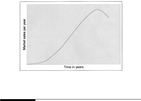
FIGURE 16-10

S-shape growth and maturity of new products.

16.5 Market Penetration

With all market forces combined and working freely, the penetration of a new technology over a period of time takes the form of an s-shaped curve shown in Figure 16-10. It is characterized by a slow initial rise, followed by a period of more rapid growth, tapering off to a saturation plateau and finally declining to make room for a newer technology. The s-shape hypothesis is strongly supported by empirical evidences.

One model available for predicting the market penetration of a new product is the diffusion model proposed by Bass.2 However, it can be argued that the renewable energy is not a really new product. It merely substitutes an existing product on a one-to-one basis. The Bass model, therefore, may not be an appropriate model for the renewable power. Since electricity is a basic need of the society, the penetration of renewable power technologies is better compared with similar substitutions in the past, such as in the steel making industry as shown in Figure 16-11. The solid lines are the actual penetration rates seen in those industries.

With ongoing developments in the wind and pv power technology and with adjustments in social attitudes, the market penetration rate may follow the line parallel to the historical experience on similar products depicted in Figure 16-11. It can be analytically represented by the Fisher and Pry substitution model.3 In this model, the rate at which the wind and pv energy may penetrate the market can be expressed as a fraction of the total MWh energy consumed every year.

© 1999 by CRC Press LLC

FIGURE 16-11

Market penetration of new product substituting existing products. Wind and pv shown in parallel with historical data.

If we let:

f = fraction of the market captured by the renewables at time t, and to = time when f equals 1⁄2

then f can be expressed as follows:

© 1999 by CRC Press LLC

Here b is the growth constant, characterizing the growth to the potential associated with a particular technology. The equation gives log-linear straight lines shown in Figure 16-11.

We take that the renewable power was successfully demonstrated to be commercially viable in the 1970s and made a commercial start in 1985. This is the time when a group of wind farms in California were installed and operated for profit by private investors. Based on this premise and based on the Fisher-Pry model just described, we draw the dotted line in Figure 16-11, beginning in 1985 and then running parallel to the historical lines followed by similar substitution products in the past. That is the rate of market penetration we can expect the wind and pv to follow in the future.

At the rate projected by the dotted line, the full 100 percent potential of the wind and pv will perhaps be realized around 2065. The wind and pv reaching the 100 percent potential in the year 2065 does not mean that they will completely replace the thermal and other power. It merely means it will reach its fully attainable potential. Experts would argue on the upper limit of this potential for a given country. However, the wind and solar, being intermittent sources of energy, cannot be the baseload provider. They may augment the baseload plants, thermal, or other types, which can dispatch energy on demand. Such reasoning puts an upper limit on the pv and wind power to well below 50 percent, perhaps around 25 percent. According to the Royal Institute of the International Affairs study published in the U.K. in May 1997, all renewable sources could provide between 25 to 50 percent of European electricity by the year 2030. The contributions of the wind and pv in the total electricity demand, however, will largely depend on the operating experience with the grid-connected plants and energy storage technologies developed during the next few decades that can remedy the nondispatchable nature of the pv and wind energy. New energy storage products are being developed that incorporate batteries, flywheel, fuel cells, and superconducting coils into system solutions for the power industry such as load leveling and power quality. Electric utility restructuring and the subsequently increased competitive market are creating new and highervalue market for energy storage. The renewable power is the new market opportunity for large-scale energy storage products.

The sophisticated prediction models have been developed by the DOE, NREL, and others based on mathematical considerations and regression analyses through applicable data. However, there is a limit to how such models can be confidently used to commit huge sums of capital investments. Small errors in data can cause large errors in projections, particularly decades out in the future. The time-proven data on how people make investment decisions under long-term uncertainties can also help. The experience indicates that investors commit funds only if the payback period is less than five years, the shorter it is, the quicker the investment penetrates. The upper limit of the payback period that starts having a significant market is four to five years, and large market penetration requires a payback period less than three years.

© 1999 by CRC Press LLC

16.6 Effect of Utility Restructuring

Although the U.S. electricity market was $210 billion in 1997, the electric utilities have grown into regulated monopolies, with no competition at the consumer level. Both the generation and the transmission of electricity remained with one company. Even when electricity could be produced by alternate sources, the transmission access to the loads was denied or the owners set the price so high that the access was effectively denied to protect their own position in the generation market.

The Public Utility Regulatory Policy Act of 1978 (PURPA) required utilities to purchase electricity from power generators using renewable energy sources or co-generation. The PURPA also required the utilities to pay the “qualifying facilities (QFs)” at rates based on their “avoided cost”. The United States Congress defined the avoided cost as the incremental cost of electrical energy the utility would incur if it generated the energy itself or purchased from another source. This definition is vague at least in one sense. That is, does the incremental cost include the share of the capital cost needed to generate the incremental unit of energy? For example, if the plant cost is taken as sunk cost, the avoided cost would primarily mean the fuel cost, which for thermal power plants may be 2 cents per kWh. On the other hand, if a new plant has to be built to meet the added demand, which a renewable power plant can supply, the avoided cost would include the capital cost of about 5 to 6 cents per kWh, making the total avoided cost of 7 to 8 cents per kWh. Congress left the exact definition of the avoided cost and the implementation of PURPA to the states. However, with the regulatory advantage of PURPA, renewable and cogeneration power plants started coming up across the nation.

Another issue debated in the renewable power industry is definition of the “avoided cost” which are paid by the utility companies. The issue is complex as illustrated by the following example. For a utility company, say the sunk cost of generation is 10 cents per kWh. This includes 2 cents for the fuel cost, and 8 cents for the capital and administrative cost of generation and transmission. If that utility has an excess capacity, its incremental avoided cost is only 2 cents, the cost of adding a customer or saving by deleting a customer. And this is what it would pay to the renewable power generator. On the other hand, it charges 12 cents/kWh to its average consumer. If the cost of selfgeneration using a wind power plant is 5 cents per kWh, the customer would save 7 cents by self-generating, but the society at large would lose 3 cents per kWh (utility would save 2 cents in fuel cost but the self-generating customer would spend 5 cents). However, in situations where the energy demand is growing but the generation and transmission capacities cannot keep up, the avoided cost includes the capital cost also. For example, Pacific Gas and Electric Company in California found that by purchasing power to meet loads at the end of heavily loaded lines, it could avoid having to construct new generation and transmission capacity. The “avoided cost” in this situation is

© 1999 by CRC Press LLC

10 cents per kWh, and the society at large would gain 5 cents (utility will save 10 cents but the self-generator would spend 5 cents). This example highlights the basic difficulty in accounting the benefits of renewable power. With such common situations, the impact of the electric utility restructuring on the renewable would depend on how fairly it is treated in defining some of the costs of both the conventional and renewable electricity.

16.6.1Energy Policy Act of 1992

By passing the Energy Policy Act of 1992, Congress encouraged even greater wholesale competition by reducing the market barriers for independent generators interested in selling electrical power. This act permits wholesale customers to have a choice of generators and obliges utilities to wheel power across their transmission lines at the same cost that they would charge to all others, including themselves. For effective implementation of the act, the utilities are required to break up the generation, transmission, and distribution businesses in separate companies. One will own the generating plants and the other will own the wires. In the past, electricity has been sold as a delivered product. The new restructuring merely unbundles the product price and the delivery charge, with the wires owned and operated separately as common carriers obligated to charge the same rate to all customers.

The new law has separated the power industry in two parts: (1) the generation and/or sale of electricity by licensed power supplier, and (2) the delivery of electricity to the consumers by regulated companies.

In the new retail competition, all customers will choose their energy suppliers, each supplier having direct open access to the transmission and distribution wires. The concept is similar to what happened to the telephone industry more than a decade ago. The idea is as old as the American free enterprise, that is the open unrestricted competition at the consumer level. The United Kingdom, Chile, Norway, and parts of Australia have systems similar to that presently taking effect in the U.S.A.

This is a major restructuring of the electrical utility industry in the U.S.A. since the beginning of the industry some 100 years ago. The uncertainty and skepticism around the EPAct of 1992 is, therefore, causing significant confusion and uncertainties of new investments in this industry.

Like PURPA, the implementation of the EPAct of 1992 is also left to individual states. The states with relatively higher energy cost (12 to 16 cents per kWh), such as California, Illinois, Massachussetts, Maine, New Hampshire, and Pennsylvania, have active pilot programs underway. In 1996, NH started a pilot project in which 16,500 customers were chosen randomly and given to choose their electricity producer. This 2-year experiment will lead to full implementation by the end of 1998. In late 1997, Pennsylvania became the largest state in the U.S.A. to implement an extensive program of competitive electric power sources. The state, home of 12 million people, has licensed 47 companies to sell power to public. Presently, there are four major established

© 1999 by CRC Press LLC

conventional utility companies (PECO Energy, PP&L Resources, GPU Energy, and Allegheny Power). Approximately one million customers volunteered for the pilot program, in which they were guaranteed savings. Full scale competition will begin in 1999, when the rate cuts will be at least 8 percent. The rate reduction is expected to reach 15 percent in the years to follow.

In Massachusetts, the most immediate effect of the restructuring is an automatic 10 percent savings effective March 1998, and 15 to 18 percent later. New Jersey plans a pilot program in 1999 and full implantation in 2003. Fact-finding and investigations are underway in mid-range cost states, but no significant activity is reported in states having lower energy cost (6 to 8 cents per kWh).

The 1992 EPAct is expected to greatly benefit the consumer. When fully implemented, the end users are expected to save 10 to 20 percent in the electricity price.4 This will be achieved partly by promoting competition among utility and nonutility power generators, and partly by the most efficient use of the generation and transmission assets by generating and wheeling the power as dictated by the regional economies. This becomes rather evident when viewed from an operational research point of view. In finding an optimized solution with constraints, the farther the constraint boundaries are, the more economical is the solution. No constraint at all results in the most economical solution.

With the expected decline in the electricity price, some of the high-cost power plants would become uneconomical compared to new power plants, including the renewables. One of the debated issues in the conventional power industry at present is who would pay the “stranded cost” of these uneconomical plants which cannot be recovered in the new competitive market. Examples of stranded costs are the cost of nuclear plants which is not recovered as yet, and the cost of locked-in power contracts with the independent generators at a higher market price. According to the Competitive Enterprises Institute, the stranded cost in the U.S. power industry is expected to add up to $200 billion.

16.6.2Impact on Renewable Power Producers

Industry leaders expect the generating business, conventional or renewable, to become more profitable in the long run under the EPAct of 1992. The reasoning is that the generation business will be stripped of regulated prices and opened to competition among electricity producers and resellers. The transmission and distribution business, on the other hand, would still be regulated. The American experience indicates that the free business has historically made more profits than the regulated business. Such is the experience in the U.K. and Chile, where the electrical power industry has been structured similar to the EPAct of 1992. The generating companies there make good profits as compared to the transmission and distribution companies.

Until the renewable electricity cost matches with the conventional one, the renewable market penetration may be slow. On the other hand, under the restructured electricity market, it is possible that the environmentally

© 1999 by CRC Press LLC

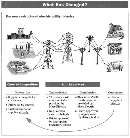
conscious consumer may choose green power even with higher prices. Surveys strongly indicate that they would.5 In 1995, several utility companies in the U.S.A. surveyed 300 customers of each. Sixty-four percent said the renewable power is very important and 36 percent said they would pay more for electricity from those sources. Twenty-four percent said they would pay at least 10 percent more. Several U.S. utilities are developing green marketing programs under which they would allow their customers to volunteer to choose to pay premium for renewable power. A pilot program, called ClearChoice was initiated in the city of San Angelo, Texas, beginning in October 1997.

As for the renewable electricity producers, they are likely to benefit as much as other producers of electricity, as they can now freely sell power to the end users through truly open access to the transmission lines (Figure 16-12).

FIGURE 16-12

New restructured electric utility industry in U.S.A. (Courtesy: Massachusetts Electric, Boston, MA.)

© 1999 by CRC Press LLC

Another benefit is that the renewable power price would be falling as the technology advances, whereas the price of the conventional power would rise with inflation, making the renewable even more advantageous in the future.

References

1.U.S. Department of Energy. 1997. “Office of the Integrated Analysis and Forecasting, International Energy Outlook 1997 with Projections to 2015,” Report No. DE-97005344, April 1997.

2.Bass, F. M. 1969. “A new product growth model,” Management Science, Vol. 15, p. 215-227, 1969.

3.Fisher, J. C. and Pry, R. H. 1971. “A simple substitution model of technological change,” Technology Forecasting and Social Change, Vol. 3, p.79-88, 1971.

4.Backus, G. and Baylis, S. 1996. “Dynamics of U.S. electrical utility deregulation,” DOE Office of Utility Technology, Report No. DE-9600052, December 1996.

5.Puttgen, H. B., Truly, R., Hyde, D. G., Walker, R., Terrado, E., Cohen, G., and Hurwitch, J. W. 1998. “Realization of alternative energy generation and storage,” IEEE Power Engineering Review, May 1998, p. 5-18.

© 1999 by CRC Press LLC