the cell produces no power at zero voltage or zero current, and produces the maximum power at voltage corresponding to the knee point of the i-v curve. This is why pv power circuits are designed such that the modules operate closed to the knee point, slightly on the left hand side. The pv modules are modeled approximately as a constant current source in the electrical analysis of the system.

Figure 8-9 is the i-v characteristic of a 22-watts panel under two solar illumination intensities, 1,000 watts/m2 and 500 watts/m2. These curves are at AM1.5 (air mass 1.5). The air mass zero (AM0) represents the condition in outer space, where the solar radiation is 1,350 watts/m2. The AM1 represents the ideal earth condition in pure air on a clear dry noon when the sunlight experiences the least resistance to reach earth. The air we find on a typical day with average humidity and pollution is AM1.5, which is taken as the reference value. The solar power impinging a normal surface on a bright day with AM1.5 is about 1,000 watts/m2. On a cloudy day, it would be low. The 500 watts/m2 solar intensity is another reference condition the industry uses to report the i-v curves.

The photoconversion efficiency of the pv cell is defined as the following:

solar power impinging the cell

Obviously, the higher the efficiency, the higher the output power we get under a given illumination.

8.6Array Design

The major factors influencing the electrical design of the solar array are as follows:

•the sun intensity.

•the sun angle.

•the load matching for maximum power.

•the operating temperature.

These factors are discussed below.

8.6.1Sun Intensity

The magnitude of the photocurrent is maximum under full bright sun (1.0 sun). On a partially sunny day, the photocurrent diminishes in direct proportion to the sun intensity. The i-v characteristic shifts downward at a lower sun

© 1999 by CRC Press LLC

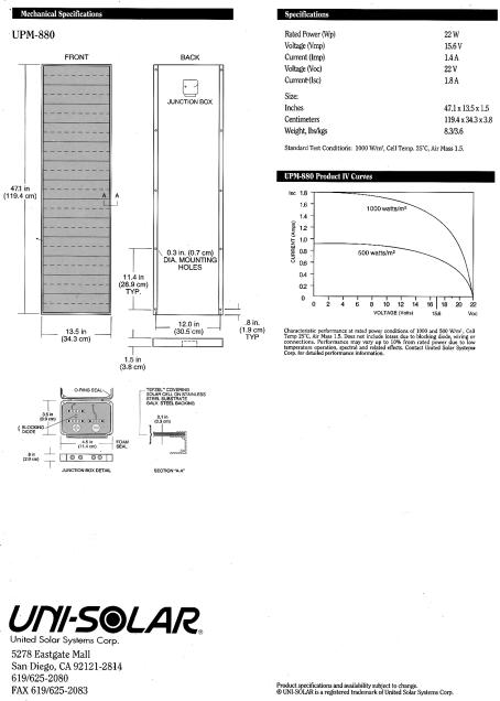
FIGURE 8-9

i-v characteristic of 22 watts pv module at full and half sun intensities. (Source: United Solar Systems Corporation, San Diego, California. With permission.)

© 1999 by CRC Press LLC

FIGURE 8-10

i-v characteristic of pv module shifts down at lower sun intensity, with small reduction in voltage.

FIGURE 8-11

Photoconversion efficiency versus solar radiation. The efficiency is practically constant over a wide range of radiation.

intensity as shown in Figure 8-10. On a cloudy day, therefore, the short circuit current decreases significantly. The reduction in the open-circuit voltage, however, is small.

The photoconversion efficiency of the cell is insensitive to the solar radiation in the practical working range. For example, Figure 8-11 shows that the efficiency is practically the same at 500 watts/m2 and 1,000 watts/m2. This means that the conversion efficiency is the same on a bright sunny day and a cloudy day. We get lower power output on a cloudy day only because of the lower solar energy impinging the cell.

8.6.2Sun Angle

The cell output current is given by I = I0 cos θ, where Io is the current with normal sun (reference), and θ is the angle of the sunline measured from the normal. This cosine law holds well for sun angles ranging from 0 to about 50°.

© 1999 by CRC Press LLC

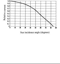
FIGURE 8-12

Kelley cosine curve for pv cell at sun angles from 0 to 90°.

TABLE 8-1

The Kelley Cosine Values of the Photocurrent

in Silicon Cells

Beyond 50°, the electrical output deviates significantly from the cosine law, and the cell generates no power beyond 85°, although the mathematical cosine law predicts 7.5 percent power generation. The actual power-angle curve of the pv cell is called Kelly cosine, and is shown in Figure 8-12 and Table 8-1.

8.6.3Shadow Effect

The array may consist of many parallel strings of series-connected cells. Two such strings are shown in Figure 8-13. A large array may get partially shadowed due to a structure interfering with the sunline. If a cell in a long-series string gets completely shadowed, it will lose the photovoltage, but still must carry the string current by virtue of its being in series with the other fully operating cells. Without internally generated voltage, it cannot produce power. Instead, it acts as a load, producing local I2R loss and heat. The remaining cells in the string must work at higher voltage to make up the loss of the shadowed cell voltage. Higher voltage in healthy cells means lower string current as per the i-v characteristic of the string. This is shown in the bottom left of Figure 8-13. The current loss is not proportional to the shadowed area, and may go unnoticed for mild shadow on a small area. However, if more cells are shadowed beyond the critical limit, the i-v curve

© 1999 by CRC Press LLC

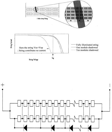
FIGURE 8-13

Shadow effect on one long pv string of an array. The power degradation is small until shadow exceeds the critical limit.

FIGURE 8-14

Bypass diode in pv string minimizes the power loss under heavy shadow.

gets below operating voltage of the string, making the string current fall to zero, losing all power of the string.

The commonly used method to eliminate the loss of string due to shadow effect is to subdivide the circuit length in several segments with bypass diodes (Figure 8-14). The diode across the shadowed segment bypasses only that segment of the string. This causes a proportionate loss of the string voltage and current, without losing the whole string power. Some modern pv modules come with such internally embedded bypass diodes.

© 1999 by CRC Press LLC