Paz R.The design of the PID controller

proportional to the error. The term Ki/s is an integral term, and the term Kds is a derivative term. Each of the terms works “independently”1 of the other.

2.1Interpretation of the Terms

We now consider each of the terms, assuming that the others are zero. With Ki = Kd = 0, we simply have u (t) = Kpe (t) . Thus at any instant in time, the control is proportional to the error. It is a function of the present value of the error. The larger the error, the larger the control signal. One way to look at this term is that the farther away from the desired point we are, the harder we try. As we get closer, we don’t try quite as hard. If we are right on the target, we stop trying. As can be seen by this analogy, when we are close to the target, the control essentially does nothing. Thus, if the system drifts a bit from the target, the control does almost nothing to bring it back. Thus enters the integral term.

Assuming now that Kp = Kd = 0, we simply have

t

u (t) = Ki e (τ) dτ

0

The addition of this integral makes the open-loop forward path of Type I. Thus, the system, if stable, is guaranteed to have zero steady-state error to a step input. This can also be viewed as an application of the internal model principle. If e (t) is non-zero for any length of time (for example, positive), the control signal gets larger and large as time goes on. It thus forces the plant to react in the event that the plant output starts to drift. We can think of the integral term as an accumulation of the past values of the error. It is not uncommon for the integral gain to be related to the proportional gain by

Ki = Kp τi

where τi is the integral time. Generally, by itself, the I term is not used. It is more commonly used with the P term to give a PI control.. The I term tends to slow the system reactions down. In order to speed up the system responses, we add the derivative term.

Assuming now that Kp = Ki = 0, we have

de (t) u (t) = Kd dt

that is that the control is based on the rate of change of the error. The more quickly the error responds, the larger the control e ort. This changing of the error indicates where the error is going. We can thus think of the derivative term as being a function

1This is not exactly true since the whole thing operates in the context of a closed-loop. However, at any instant in time, this is true and makes working with the PID controller much easier than other controller designs.

where constants ap and ad are as yet undetermined. Each of the terms thus has a di erent “error” associated with it. Note that when ap = ad = 1, that we have the original PID design. Note also that when r (t) is a piecewise constant signal (only step changes), then for all time (except at the actual step locations), r˙ (t) = 0, and thus,

which is independent of r (t) and ad. In general, since y is the output of the plant, it will be a smooth function and thus y˙ will be bounded. It is thus not uncommon to let

ad = 0. This eliminates spikes in the term Kd ded(t) , without substantially a ecting the

dt

overall control performance.

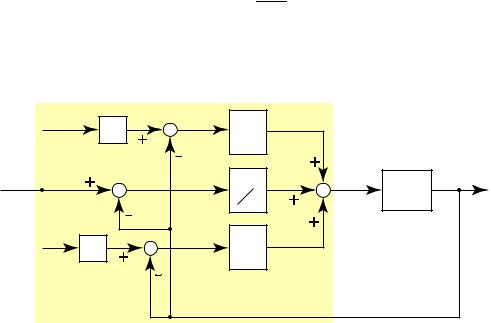
A block diagram for this is shown. As it appears, it seems much more complicated. However, it is actually not much more complicated.

Figure 2: The Setpoint Weighting Configuration

As we have seen, changing ad doesn’t change the overall design. Changing ap, however, may change the design. The rationale behind ap is that if, for example, ap = 0.5, then a large step change in r (t) doesn’t create such a large control magnitude. However, in general, ep does not go to zero when y = r. Thus, there is a persistent control applied even when it is not necessary. The use of this, then is of questionable value. Setting ap = 1, however, brings us back to the original error.

2.3Overall Usage

The PID controller performs especially well when the system has first order dynamics (a single pole). Actually, in this case, the P controller is a state-feedback control! In

6

general, for the system with first-order dynamics the PI control is su cient, and the D is not needed.

For the system with essentially second-order dynamics, the PD control corresponds to state feedback. The PID control generally works well for these systems.

The PID controller can also work for some systems of higher order. Generally speaking, the derivative term is beneficial when the time constants of the system di er by orders of magnitude. It is sometimes helpful when tight control of higher-order dynamics is required. This is because the higher order dynamics prevent the use of high proportional gain. The D provides damping and speeds up the transient response.

The PID controller, of course, is not the end-all of controllers. Sometimes the controller just won’t work very well. The following are cases when the PID control doesn’t perform well. In general, these require the use of more sophisticated methods of control.

•Tight control of higher order process

•Systems with long delay times. In this case, the derivative term is not helpful. A “Smith predictor” is often used in this case.

•Systems with lightly damped oscillatory modes

•Systems with large uncertainties or variations.

•Systems with harmonic disturbances

•Highly coupled multi-input, multi-output systems—especially where coordination is important.

2.4Example

num=20*[1 2];den=conv([1 .5],[1 1 4]);

Kp=9;Ki=4;Kd=2;t1=1/100;

numc=[Kp*t1+Kd,Kp+Ki*t1,Ki]/t1;denc=[t1,1,0]/t1;

numf=conv(num,numc);denf=conv(den,denc);

dencl=denf+[0 0 numf];

numy=numf;

syso=tf(num/20,den);sysy=tf(numy,dencl);

t=[0:.002:10]’;

yo=step(syso,t);yc=step(sysy,t);

figure(1);plot(t,[yo yc]);grid

xlabel(’time (sec)’);ylabel(’y(t)’)

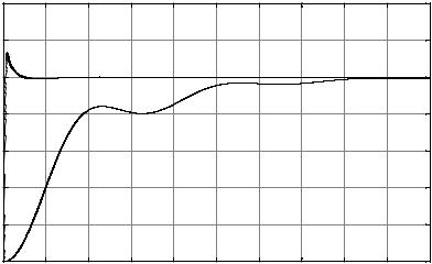
We thus obtain the plot shown. This plot compares the open-loop response with that of the PID controlled response. For the open-loop, we simply scaled the step input so that the overall system output settled out to 1.

Figure 3: Step Response for PID and Open-Loop Systems

We see that the PID controlled system performs much better than the open loop. It is often advantageous to make a comparison with the open-loop system, since that shows what would happen using the simplest kind of control. Indeed, the open loop requires no sensors and is thus much less costly to build and maintain than the PID system. If the PID system did not perform so much better, it might not be worthwhile.

8

3Plant Modeling

In general, the more we know about a system, the better we will be able to control it. If we know nothing about a system, we better not be trying to control it. A logical question, then, is how much (or little) do we need to know, and how will we obtain that data?

3.1Information Required

The more information available about the system, the better it can be controlled2. Many processes to be controlled are either di cult to model or else it is di cult to obtain the parameters for the model. For example, the dynamic inductance of a dc motor is very di cult to obtain. Generally, to obtain a model, it is necessary to perform some experiments to obtain actual parameter values. The type of experiments will determine what data is obtained. Here, we consider three types of experiments. Each will give a di erent type of information. That information will be used to design the PID controller.

In general, the experiments to be performed require that the system be stable. If not, the experiments won’t work. This, of course, is a great restriction. Unless the exact model of the unstable system is known, there is no known way to tune a PID controller. Some controllers, such as adaptive controllers are able to compensate for unstable systems, however their complexity excludes them from consideration in this course.

3.2Step Response Information

A simple experiment to perform is the step response test. Here, we assume a unit step is applied to the system, although it is also possible to scale the whole experiment is necessary. From the results of this test, the data may be used to obtain approximations of the system.

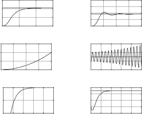
Figure 4 shows example step responses for a number of di erent possibilities. The tuning rules were essentially developed for a step response of type A. The rules, however, may work for responses of type B and E. The responses C and D are for unstable systems. If the plant is exactly known, it might be possible to design a PID controller, but there is no guarantee. As for the system with response F, the system has a zero in the RHP (unstable zero). A PID controller may reduce the settling time of the system, but is likely to accentuate the undershoot.

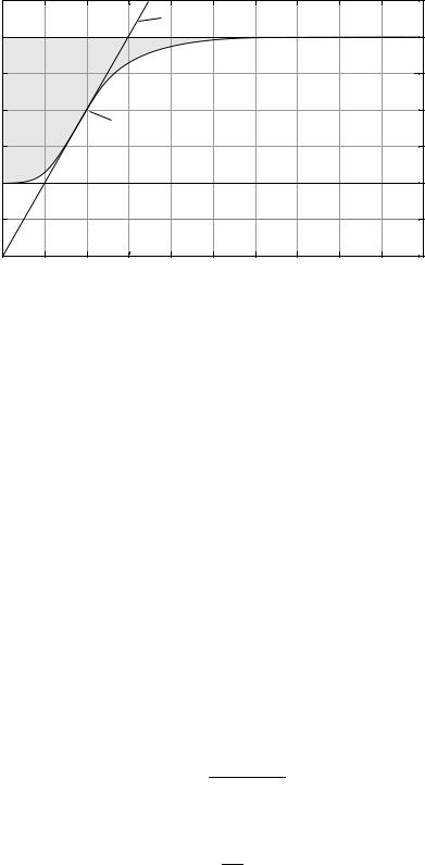
The PID controller rules are thus essentially designed for a first or second-order, nonoscillatory system with possibly some time-delay. An example plot is shown in Figure 5.

The step response has several values that are of importance in obtaining an approximate transfer function for the system. First, we see yss which is the steady-state value for the step input. Next, we see y0, τ0, and m, which gives a linear approximation of the

2There are limits, of course, as to what can be achieved.

Figure 4: Six Possible Step Responses

10

Figure 5: A Typical Step Response

transient portion of the step response. Given only the step response data, we first find the point at which the derivative of y is at a maximum. This value is y˙max and occurs at time tmax. The equation of the line that passes through the point y (tmax) with slope m = y˙max is given by

Here, τ0 is often called the apparent dead time. In this case, we may approximate the plant by the model

which doesn’t match the steady-state characteristics very well, but does match the transient portion in a linear fashion. A model that approximates the system’s steady-state behavior is given by