

Paz R.The design of the PID controller
.pdf3. PLANT MODELING |
11 |
and where A0 is the area between yss and y (t)
∞
A0 = |yss − y (t)| dt (1.16)
0
Note that even though the integral is all the way to ∞, actually the integral may be approximated for a shorter time since the di erence |yss − y (t)| becomes small after a certain point. The approximation Ga2 generally doesn’t match the transient portion extremely well, but is a good first-order approximation. It has been observed that the quantity
κ1 = |
τ0 |
(1.17) |
τar |
is a measure of the di culty of control. Generally 0 ≤ κ1 ≤ 1, and the closer κ1 is to 1, the more di cult the system is to control using the PID. Still another approximation is given by
Ga3 (s) = (yss) |
e−τ 0s |
|
(1.18) |
1 + τats |
|||
where |
|
|
|
τat = τar − τ0 |
(1.19) |
||
is called the apparent time constant. This is the better of the three approximations. Generally speaking, τat is less susceptible to noise in the step response.
3.3Frequency Response Information
Another type of experiment that actually provides more useful (in terms of designing the PID controller) information is a frequency response test. Here, we do a simple test. Again, we assume that the system is stable. We also let r (t) = ε, a very small value.
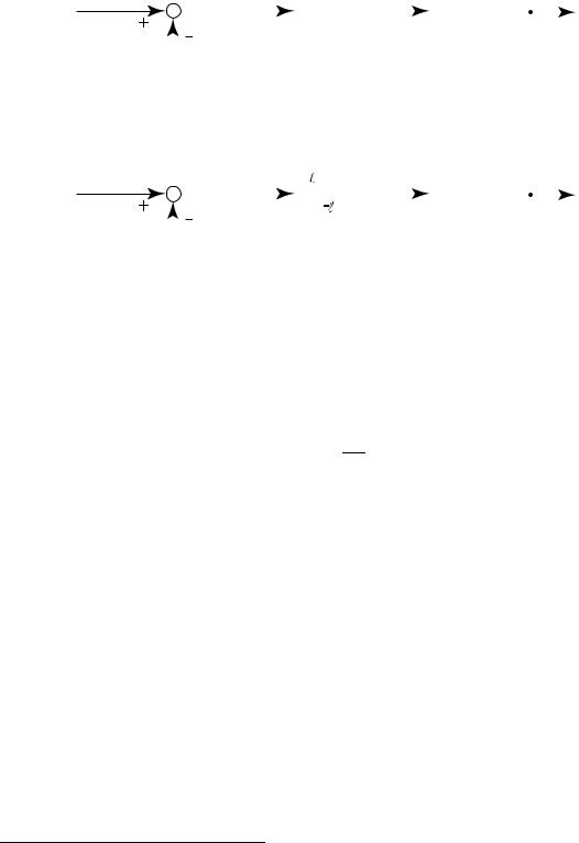
There are two variations on the Frequency response tests. Both yield essentially the same information. The first test, illustrated in Figure 6(a) is that of a P controller. Here, the gain Kp is increased from zero until the system begins to oscillate. When Kp is set such that there is a constant oscillation (neither increasing nor decreasing), that value is called the ultimate gain and is denoted Ku. The oscillation will generally be periodic with some period Tu.
This approach is generally risky since the plant is operated near instability. Also, generally, it is di cult to keep the control amplitude bounded (important for safety!). Thus, in general, this method is di cult to automate.
The second variation is based on the diagram in Figure 6(b). Here, a relay is employed, giving the control signal
, e (t) ≥ 0
u (t) = (1.20)
− , e (t) < 0
This control, for most systems of interest, will result in an oscillation. Eventually the control input will be a square wave of amplitude , and have a period approximately
12
R(s) |
E(s) |
|
|
Kp |
U(s) |
|
Y(s) |
|||||||
|
|
G(s) |
||||||||||||
|
|
|
|
|
|
|
|
|
|
|
||||
|
|
|
|
|
|
|
|
|
||||||
|
|
|
|
|
|
|
|
|
|
|
|
|
|
|
|
|
|
|
|
|
|
|
|
|
|
Plant |
|
|
|
|
|
|
|
|
|
|
|
|
|
|
|
|
|
|
|
(a) |
|
|
|
|
|
|
|
|
|
|
|
|
|
|
|
|
|
|
|
|
|
|
|
|
|
|
|
|
(b) |
|
|
|
|
|
|
|
|
|
|
|
|
||
R(s) |
E(s) |
|
|
|
|
|
U(s) |
|
Y(s) |
|||||
|
|
|
|
|
G(s) |
|||||||||
|
|
|
|
|
||||||||||
|
|
|
|
|
|
|
|
|
|
|
|
|
||
|
|
|
|
|
|
|
|
|
|
|
|
|
|
|
|
|
|
|
|
|
|
|
|
|
|
|
|
|
|
|
|
|
|
|
Relay |
Plant |
|
|
||||||
|
|
|
|
|
|
|
|
|
|
|
|
|
|
|
Figure 6: Frequency Response Test Setups
equal to Tu from the previous version of the test. The output of the system will settle out to be a sinusoid of amplitude α. In this case, we may obtain the ultimate gain from the formula3
4
Ku = πα (1.21)
This Ku and Tu are close to the actual values of Ku and Tu found in the previous variation, the previous values being actually more accurate.
Thus, regardless of which variation we choose, we end up with Tu and Ku. The nice thing about this test is that the control signal is bounded for all time. The threat of instability is also reduced.
3.4System Identification
System Identification is a method of obtaining a transfer function by applying a known test signal to a system, observing the output, and comparing it with the input to determine the transfer function of the system. This test is generally quite a bit more involved than either the step response test or the frequency response test. It yields, however, an actual transfer function, rather than just a few values of an approximate transfer function.
Because of the complexity, this topic will not be considered here, but will be relegated to another course.
3This value is obtained by a type of nonlinear analysis called describing functions.
3. PLANT MODELING |
13 |
3.5Example
Consider the plant
G (s) = |
10000 |
(1.22) |
s4 + 126s3 + 2725s2 + 12600s + 10000 |
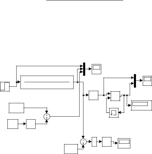
We use the following SIMULINK model to perform the step response experiment. Note that in this setup, we have blocks added to help compute the necessary constants. Performing the simulation once, we obtain
y˙max = 0.6632 |
(1.23) |
This value is plugged back into the diagram.
|
|
Scope |
|
|
|
|
10000 |
|
|
|
|
|
s4+126s3+2725s2+12600s+10000 |
y(t) |
|
|
Scope2 |
|
Transfer Fcn |
y(t) |
|
|
|
|
|
|
|
||
Step |
|
|
|
|
|
|
du/dt |
|
max |
|
|
|
|
ydot |
|
||
y0 |
|
|
|
|
|
|
Derivative |
MinMax |
0.6632 |
||
|
|
|
|
|
|
.1076 |
|
|
|
|
|
|
|
|
|
|
ydotmax |
|
1 |
|
|
Memory |
|
.6632 |
|
|
|
|
|
s |
|
|
|
|
|
|
|
|
|
|
|
MaxYdot |
Integrator1 |
|
|
|
|
|
|
|u| |
1 |
|
1.26 |
|
|
s |
|
||
|
|
|
|
|
|
|
1 |
Abs |
Integrator |
A0 |
|
|
yss |
|
|
|
|
Figure 7: SIMULINK Diagram for the Step Response Test
In addition, looking at Scope2, we can find the time at which the maximum slope occurs. Zooming in, we obtain
tmax = 0.5 |
(1.24) |
Zooming into Scope, we find that
y (tmax) = y (0.5) = 0.224 |
(1.25) |

14
From this we may calculate
y0 = |
(y˙max) (tmax) − y (tmax) |
|
= |
(0.6632) (0.5) − (0.224) = 0.1076 |
(1.26) |
This is also plugged back into the diagram. We also compute
τ0 |
= |
y0 |
= |
0.1076 |
= 0.1622 |
(1.27) |
y˙max |
|
|||||
|
|
0.6632 |
|
|
||
We note from Scope that yss = 1. This is plugged back into the diagram and the simulation is performed again. Doing so, we find the line displayed as in Figure 5 in Scope. We also obtain the integral value
A0 = 1.26 |
(1.28) |
We thus may compute
τar |
= |
|
A0 |
= |
1.26 |
= 1.26 |
||
|
|
1 |
||||||
|
|
|
yss |
|
|
|||
τat |
= |
τar − τ0 = 1.26 − 0.1622 = 1. 0978 |
||||||
and find that |
|
|
|
|
0.1622 |
|
||
|
|
|
κ1 = |
= 0. 1287 |
||||
|
|
|
|
|
||||
|
|
|
1.26 |
|||||
indicating that this system is not too hard to control using a PID controller. For the Frequency Response Test, we use the following SIMULINK diagram.
(1.29)
(1.30)
(1.31)
|
|
|
|
|
|
|
|
|
|
|
|
|
|
|
|
|
|
|
|
|
|
|
|
|
|
|
|
|
|
|
|
|
|
|
|
|
|
|
|
|
|
|
|
|
|
|
|
|
|
|
|
|
|
|
|
|
|
|
|
|
|
|
|
|
|
|
|
|
|
|
|
|
|
|
|
|
|
|
|
|
|
|
|
|
|
|
|
|
|
|
|
|
|
|
|
|
|
|
|
|
|
|
|
|
|
|
|
|
|
|
Scope1 |
|
|
|
|
|
|
||||||
|
|
|
|
|
|
|
|
|
|
|
|
|
|
|
|
|
|
|
|
|
|
|
|
|
|
|
|
|
|
|
|
|
|
|
|
|
|
|
|
|
|
|
|
|
|
|
|
10000 |
|
|
|
|
|
|
|
|
|
|
|||
|
0 |
|
|
|
|
|
|
|
|
|
|
|
|
|
|
|
|
|
|
|
|
|
|
|
|
|||||
|
|
|
|
|
|
|
|
|
|
|
|
|
|
|
|
|
s4+126s3+2725s2+12600s+10000 |
|
|
|
|
|
|
|||||||
|
|
|
|
|
|
|
|
|
|
|
|
|
|
|
|
|
|
|
|
|
|
|
|
|
|
|
|
|
|
|
Constant |
|
|
Relay |
|
|
|
|
|
|
|
|
|
|
|
|
Scope |
||||||||||||||
|
Transfer Fcn |
|||||||||||||||||||||||||||||
|
|
|
|
|
|
|
|
|
|
|
|
|
|
|
|
|
|
|
|
|
|
|
||||||||
|
|
|
|
|
|
|
|
|
|
|
|
|
|
|
|
|
|
|
|
|
|
|
|
|
|
|
|
|
|
|
Figure 8: SIMULINK Frequency Response Test Configuration
This is simulated for 100 seconds. The relay has amplitude = 1. Looking at either Scope or Scope1, we find the period of oscillation to be
Tu ≈ 0.64 |
(1.32) |
4. PID TUNING |
|
|
|
|
|
15 |
|
and looking near t = 100, at Scope, we find that the steady-state amplitude is |
|||||||
|
|
α = 0.0527 |
|
(1.33) |
|||
From this we find the ultimate gain |
|
|
|
|
|
|
|
4 |
4 (1) |
|
|
||||
Ku ≈ |
|
= |
|
|
|
= 24.16 |
(1.34) |
πα |
π (0.0527) |
||||||
Note that the actual values for this are Tu = |
2π |
= 0.6283, and Ku = 101 |
= 25.25.4 |
||||
|
|||||||
|
|
10 |
|
4 |
|
||
4PID Tuning
Having obtained a basic system information, from either of the tests, we are now in a position to perform some designs on the system. These designs are based upon the data obtained by the above experiments.
4.1Ziegler-Nichols Step Response Method
This is the earliest design method for the PID controller. It was originally developed in 1942, so its not exactly state-of-the-art. It does, however, work e ectively for many systems. This method is based on the approximate model Ga1 (s) . Once this model has been determined by the step response test, we may design controllers according to the following table. Note that only y0 and t0 are used.
Controller |
|
Kp |
|
|
Ki |
Kd |
|||||
PI |
|
9 |
|
|
|
3 |
|
|
0 |
||
|
10y0 |
|
10y0τ0 |
||||||||
|
|
|
|
||||||||
PID |
|
6 |
|
|
|
3 |
|
|
3τ0 |
||
|
|
5y0 |
|
|
5y0τ0 |
5y0 |
|||||
|
|
|
|
|
|||||||
These formulae are heuristic rules based upon the response of many di erent systems. The design criteria was to ensure that the amplitude of closed-loop oscillation decay at a rate of 1/4. This is actually often too lightly damped. It is also often too sensitive.
4.2Ziegler-Nichols Frequency Response Method
From the Frequency Response Test (or Relay Test), we obtained the ultimate gain Ku and Tu. From these values, we obtain the following table.
|
Controller |
Kp |
|
Ki |
Kd |
||
|
PI |
2Ku |
|
Ku |
|
0 |
|
|
5 |
|
2Tu |
||||
|
|
|
|
|
|||
|
PID |
3Ku |
6Ku |
3KuTu |
|||
|
5 |
|
5Tu |
40 |
|||
|
|
|
|
||||
|
|
|
|
|
|
|
|
4These were obtained analytically because we actually know the system exactly. They are close enough to the approximations which don’t require exact knowledge to obtain.
16
We note that in this case as in the previous case,
KiKd |
= |
1 |
(1.35) |
|
K2 |
4 |
|||
|
|
|||
p |
|
|
|
This appears to be common in PID tuning. Both methods also often give too high a Kp, which is related to the designed decay ratio. The ZNSR method generally gives a higher Kp than the ZNFR method.
4.3Chein-Hrones-Reswick Method
A modification of the Ziegler-Nichols method is the Chein-Hrones-Reswick (CHR) method. This is based more on a setpoint response. This is a step-response method and uses y0, τ0 and τat. In this case, we have the following table.
Controller |
|
Kp |
|
|
Ki |
|
Kd |
||||||
PI |
|
7 |
|
|
|
7 |
|
|
0 |
|
|||
|
20y0 |
|
24y0τ at |
|
|||||||||
|
|
|
|
|
|
||||||||
PID |
|
3 |
|
|
|
3 |
|
|
|
3τ0 |
|
||
|
|
5y0 |
|
|
5y0τ at |
|
10y0 |
||||||
|
|
|
|
|
|
||||||||
4.4Example
Consider the example given in the previous section. Here, we consider only PID controllers. There, we obtained the values y0 = 0.1076, τ0 = 0.1622, τat = 1. 0978, Tu ≈ 0.64, and Ku ≈ 24.16. We thus obtain the controller designs
Controller |
Kp |
Ki |
Kd |
ZNSR |
11.1524 |
34.3786 |
0.9045 |
|
|
|
|
CHR |
5.5762 |
5.0794 |
0.4522 |
|
|
|
|
ZNFR |
14.496 |
45.300 |
1.1597 |
|
|
|
|
MATLAB is used to perform the simulations of the systems. We thus obtain the plot shown below. We note that the CHR design is the best overall. That is partially due to the fact that it is tailored to the setpoint problem.

5. INTEGRATOR WINDUP |
17 |
1.6 |
|
|
|
|
|
|
|
|
|
|
1.4 |
|
|
|
|
|
|
|
OpenLoop |
|
|
|
|
|
|
|
|
|
ZNSR |
|
|
|
1.2 |
|
|
|
|
|
|
|
CHR |
|
|
|
|
|
|
|
|
|
ZNFR |
|
|
|
|
|
|
|
|
|
|
|
|
|
|
1 |
|
|
|
|
|
|
|
|
|
|
0.8 |
|
|
|
|
|
|
|
|
|
|
0.6 |
|
|
|
|
|
|
|
|
|
|
0.4 |
|
|
|
|
|
|
|
|
|
|
0.2 |
|
|
|
|
|
|
|
|
|
|
0 |
|
|
|
|
|
|
|
|
|
|
0 |
0.5 |
1 |
1.5 |
2 |
2.5 |
3 |
3.5 |
4 |
4.5 |
5 |
|
|
|
|
|
time |
|
|
|
|
|
Figure 9: Example Step Responses
5Integrator Windup
In general, the actuator for any system is limited, i.e., there is a maximum exertion that the actuator can accomplish. If the actuator is a power amplifier, it generally has “rails.” Thus, the design for a linear system is not su cient since the real system is not linear, but has a nonlinear saturation term. A controller designed for a linear system will often not work on a nonlinear system. This configuration is illustrated below. Here, a disturbance input is also added.
|
|
|
|
|
|
|
|
|
|
|
|
|
Disturbance |
|||||
|
|
E(s) |
|
|
|
|
|
|
|
|
|
|
W(s) |
|||||
|
|
|
|
|
|
|
|
|
|
|
|
|||||||
R(s) |
|
U(s) |
|
|
|
|
|
V(s) |
|
|
|
|
Y(s) |
|||||
C(s) |
|
|
|
|
|
|
|
G(s) |
|
|||||||||
|
|
|
|
|
|
|
|
|
|
|
|
|
|
|
|
|
||
|
|
|
|
|
|
|
|
|
|
|
|
|
|
|
|
|
||
|
|
|
|
|
|
|
|
|
|
|
|
|
|
|
|
|
|
|
|
|
Controller |
Saturation |
|
|
Plant |
|
|
|
|||||||||
|
|
|
|
|
|
|
|
|||||||||||
|
|
|
|
|
|
|
|
|
|
|
|
|
|
|
|
|
|
|
Figure 10: Nonlinear System with Disturbance
When the actuator saturates, the loop is e ectively open. In particular, if the control
18
is such that a long period of saturation exists, it is possible for the integral term to keep integrating even when it is not reasonable to do so. the integrator itself is open-loop unstable, and the integrator output will drift higher. This is called integrator windup. In order for the integrator to “unwind,” the error signal must actually change sign before the output of the integrator will start to return to zero. Thus, the actuator remains saturated even after error changes sign since the controller’s output stays high until the integrator resets.
This is di cult to visualize, so we give our example next.
5.1Example
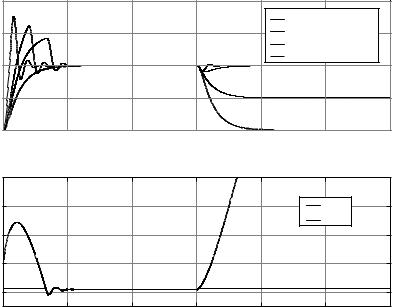
Consider the problem of the previous example, using the ZNSR method. Suppose we have a saturation limit where we may have = 1, 1.5, 2 or 5. Suppose also that the disturbance w (t) is a negative unit step input that turns on at time t = 15. A plot of this is shown below, and is compared with the open-loop system. Note that the open-loop system goes to zero after the disturbance enters because the disturbance “cancels” the reference signal.
|
2 |
|
|
|
|
|
|
|
|
|
|
|
|
=1.5 |
|
|
1.5 |
|
|
|
|
=2 |
|
|
|
|
|
|
|
=5 |
|
(t) |
1 |
|
|
|
|
=1&openloop |
|
|
|
|
|
|
|
||
y |
|
|
|
|
|
|
|
|
0.5 |
|
|
|
|
|
|
|
0 |
|
|
|
|
|
|
|
0 |
5 |
10 |
15 |
20 |
25 |
30 |
|
|
|
|
time |
|
|
|
|
40 |
|
|
|
|
|
|
|
30 |
|
|
|
|
u(t) |
|
) |
|
|
|
|
|
v(t) |
|
(t),v(t |
20 |
|
|
|
|
|
|
|
|
|
|
|
|
||
|
|
|
=1.5 |
|
|
|
|
u |
10 |
|
|
|
|
|
|
|
|
|
|
|
|
|
|
|
0 |
|
|
|
|
|
|
|
0 |
5 |
10 |
15 |
20 |
25 |
30 |
|
|
|
|
time |
|
|
|
|
Figure 11: Integrator Windup E ects when = 1, 1.5, 2, 5 |
||||||
When = 1, the control signal quickly saturates and thus the system behaves essentially as the open-loop system. We have shown the control signal u (t) and the actuation

5. INTEGRATOR WINDUP |
19 |
signal v (t) for = 1.5 in the bottom graph. Here, the input immediately saturates, but finally resets at around t = 3, in which case the system begins to act like a linear system. When the disturbance comes, the integrator again saturates the actuator, and the integrator value drives u (t) o to infinity, never to return. The net e ect on the output is that the output does not return to the setpoint value, but settles at 0.5. This is better than the case of = 1, however. For ≥ 2, the system recovers from the disturbance and continues tracking. When = 5, the output looks identical to the original ZNSR response.
5.2Back Calculation
The idea of an anti-windup technique is to mitigate the e ects of the integrator continuing to integrate due to the nonlinear saturation e ect. In the Back-Calculation method, when the actuator output saturates, the integral is recomputed such that its output keeps the control at the saturation limit. This is actually done through a filter so that anti-windup is not initiated by short periods of saturation such as those induced by noise.
This method can be viewed as supplying a supplementary feedback path around the integrator that only becomes active during saturation. This stabilizes the integrator when the main feedback loop is open due to saturation. In this case, we have the setpointweighted control law
u (t) = Kpep (t) + 0 |
t |
|
ded (t) |
|
|
e¯i (τ) dτ + Kd |
|||
|
dt |
|
||
where
ep = apr (t) − y (t) , ed (t) = adr (t) − y (t)
and where we have the integral error
1
e¯i (t) = Ki (r (t) − y (t)) + Tt (v (t) − u (t))
(1.36)
(1.37)
(1.38)
Note that if there is no saturation, then v (t) = u (t) and e¯i corresponds to ei given previously. When v (t) = u (t) , then the tracking time constant Tt determines how quickly after saturation the integrator is reset.
In general, the small Tt is better as it gives a quicker reset. However, if it is too small, noises may prevent it from actually resetting the integrator. As a general rule, we choose
τd < Tt < τi |
(1.39) |
where τd is the derivative time and τi is the integral time referred to earlier. A typical choice will be
(1.40)
20
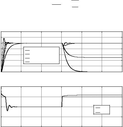
We revisit the previous example. In this case, we use the Back-Calculation in performing the integration, with
|
|
|
Tt = √τdτi = |
Kd |
|
(1.41) |
|
|
|
|
|
|
Ki |
|
|
again with = 1, 1.5, 2 and 5. A plot of the response is shown below. |
|
||||||
|
1.4 |
|
|
|
|
|
|
|
1.2 |
|
|
|
|
|
|
y(t) |
1 |
|
|
|
|
|
|
0.8 |
|
=1.5 |
|
|
|
|
|
|
0.6 |
|
=2 |
|
|
|
|
|
0.4 |
|
=5 |
|
|
|
|
|
|
=1&openloop |
|
|
|
|
|
|
0.2 |
|
|
|
|
|
|
|
|
|
|
|
|
|
|
|
0 |
5 |
10 |
15 |
20 |
25 |
30 |
|
0 |
||||||
|
|
|
|
time |
|
|
|
|
2 |
|
|
|
|
|
|
) |
1.5 |
|
=1.5 |
|
|
|
|
|
|
|
|
|
|
||
),v(t |
|
|
|
|
|
|
|
|
|
|
|
|
|
|
|
u(t |
1 |
|
|
|
|
u(t) |
|
|
0.5 |
|
|
|
|
v(t) |
|
|
|
|
|
|
|
|
|
|
0 |
5 |
10 |
15 |
20 |
25 |
30 |
|
0 |
||||||
|
|
|
|
time |
|
|
|
Figure 12: Back-Calculation Responses
Here, we see that for = 1, there is e ectively no change in the response. This is because the saturation is so close to the boundary for the step input that there is no “headroom.”
For = 1.5, we also have a comparable disturbance response to that above. This is due to the fact that the combination of the setpoint and the disturbance are past the saturation limit. We note, however, two beneficial aspects of the back-calculation. The first is that the response to the initial setpoint change is significantly better than when the back-calculation is not used. We have virtually no overshoot, and a much faster settling time. This is because the back-calculation resists the tendency of the controller to initially saturate. The second benefit is that when the disturbance hits, the control signal u (t) does not head o to infinity, but remains bounded.
For ≥ 2, we see a comparable disturbance rejection to that of the original problem. However, as with the = 1.5 case, we see a significantly improved transient response to