solved the problem by changing the data model to make it simpler. Before leaving this example, let us summarize what we have learned:

In header/detail models, the header table acts as both a dimension and a fact table at the same time. It is a dimension to slice the detail, and it is a fact table when you need to summarize values at the header granularity.

If you summarize values from the header, any filters from dimensions linked to the detail are not applied unless you activate bidirectional filtering or you use the many-to-many pattern.

Both bidirectional filtering and the bidirectional DAX pattern summarize the values at the header granularity, leading to totals that do not sum. This might or might not be an issue. In this example, it was an issue and we had to fix it.

To fix the problem of additivity, you can move the total values stored in the header table by allocating them as percentages to the detail table. Once the data is allocated to the detail table, it can be easily summed and sliced by any dimension. In other words, you denormalize the value at the correct granularity to make the model easier to use.

A seasoned data modeler would have spotted the problem before building the measure. How? Because the model contained a table that was neither a fact table nor a dimension, as we saw at the beginning. Whenever you cannot easily tell whether a table is used to slice or to aggregate, then you know that the danger of complex calculations is around the corner.

Flattening header/detail

In the previous example, we denormalized a single value (the discount) from the header to the detail by first computing it as a percentage on the header and then moving the value from the header to the detail. This operation can be moved forward for all the other columns in the header table, like StoreKey, PromotionKey, CustomerKey, and so on. This extreme denormalization is called flattening because you move from a model with many tables (two, in our case) to one with a single table containing all the information.

The process of flattening a model is typically executed before the data is loaded into the model, via SQL queries or M code, using the query editor in Excel or Power BI Desktop. If you are loading data from a data warehouse, then it is very likely that this process of flattening already happened before the data was moved to the data warehouse. However, we think it is useful to see the differences between querying and using a flat model against a structured one.

Warning

In the example we used for this section, we did something weird. The original model was already flattened. On top of this, for educational purposes, we built a structured model with a header/detail. Later, we used M code in Power BI Desktop to rebuild the original flat structure. We did it to demonstrate the process of flattening. Of course, in the real world, we would have loaded the flat model straight in, avoiding this complex procedure.

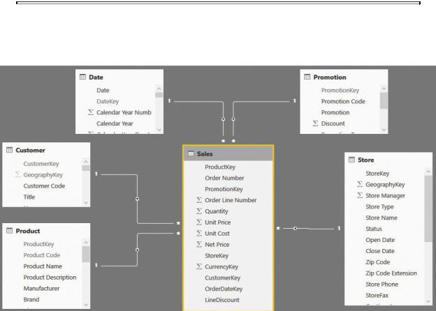
The original model is the one previously shown in Figure 2-1. Figure 2-9 shows the flattened model, which is basically a pure star schema with all the columns from SalesHeader denormalized in Sales.

FIGURE 2-9 Once flattened, the model again becomes a pure star schema.

The following steps are carried out in the query that loads the Sales table:

1.We joined SalesHeader and SalesDetail together based on Order Number, and we added the related columns of Sales Header to Sales.

2.We created a new hidden query that computes, out of Sales Detail, the total order, and we joined this query with Sales to retrieve the total order.

3.We added a column that computes the line discount the same way we did it

in the previous example. This time, however, we used M code instead of DAX.

When these three steps are complete, you end up with a perfect star schema that offers all the advantages of a star schema. Flattening foreign keys to dimensions, like CustomerKey and OrderDateKey, is straightforward because you simply make a copy of the value. However, flattening metrics like the discount typically requires some kind of reallocation, as we did in this example by allocating the discount as the same percentage on all the lines. (In other words, it is allocated using the line amount as the allocation’s weight.)

The only drawback of this architecture is that whenever you need to compute values based on columns that were originally stored in the header, you need to pay attention. Let us elaborate on this. If you wanted to count the number of orders in the original model, you could easily create a measure like the following one:

Click here to view code image

NumOfOrders := COUNTROWS ( SalesHeader )

This measure is very simple. It basically counts how many rows are visible, in the current filter context, in the SalesHeader table. It worked because, for SalesHeader, there is a perfect identity between the orders and rows in the table. For each order, there is a single line in the table. Thus, counting the rows results in a count of the orders.

When using the flattened model, on the other hand, this identity is lost. If you count the number of rows in Sales in the model in Figure 2-9, you compute the number of order lines, which is typically much greater than the number of orders. In the flat model, to compute the number of orders, you need to compute a distinct count of the Order Number column, as shown in the following code:

Click here to view code image

NumOfOrders := DISTINCTCOUNT ( Sales[Order Number]

)

Obviously, you should use the same pattern for any attribute moved from the header to the flat table. Because the distinct count function is very fast in DAX, this is not a typical issue for medium-sized models. (It might be a problem if you have very large tables, but that is not the typical size of self-service BI models.)

Another detail that we already discussed is the allocation of values. When we moved the total discount of the order from the header to the individual lines, we allocated it using a percentage. This operation is needed to enable you to

aggregate values from the lines and still obtain the same grand total, which you might need to do later. The allocation method can be different depending on your specific needs. For example, you might want to allocate the freight cost based on the weight of the item being sold instead of equally allocating it to all the order lines. If this is the case, then you will need to modify your queries in such a way that allocation happens in the right way.

On the topic of flattened models, here is a final note about performance. Most analytical engines (including SQL Server Analysis Services, hence Power BI and Power Pivot) are highly optimized for star schemas with small dimensions and large fact tables. In the original, normalized model, we used the sales header as a dimension to slice the sales detail. In doing this, however, we used a potentially large table (sales order header) as a dimension. As a rule of thumb, dimensions should contain fewer than 100,000 rows. If they grow larger, you might start to notice some performance degradation. Flattening sales headers into their details is a good option to reduce the size of dimensions. Thus, from the performance point of view, flattening is nearly always a good option.

Conclusions

This chapter started looking at different options to build a data model. As you have learned, the same piece of information can be stored in multiple ways by using tables and relationships. The information stored in the model is identical.

The only difference is the number of tables and the kind of relationships that link them. Nevertheless, choosing the wrong model makes the calculation much more complex, which means the numbers will not aggregate in the expected way.

Another useful lesson from this chapter is that granularity matters. The discount as an absolute value could not be aggregated when slicing by dimensions linked to the line order. Once transformed into a percentage, it became possible to compute the line discount, which aggregates nicely over any dimension.