

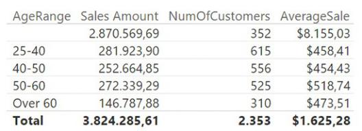
FIGURE 5-27 With a proper dimension, you can easily slice by age range.
You can obtain a good data model by separating the rapidly changing attribute from the original dimension and storing it as a value in the fact table or, if needed, building a proper dimension on top of the attribute. The resulting loading process is much easier—and the data model is much simpler—than with a fully featured SCD.
Choosing the right modeling technique
In this chapter, we have shown two different methods for handling changing dimensions. The canonical way is to create a fully featured SCD with a rather complex loading process. The simpler way is to store the slowly changing attribute as a column in the fact table, and, if needed, to build a proper dimension on top of the attribute.
The latter solution is much simpler to develop, so sometimes it will be the best way to handle SCDs, especially if you can easily isolate one slowly changing attribute. However, if the number of attributes is larger, you might end up having too many dimensions, making the data model difficult to browse. As often happens in data modeling, you should always think carefully before choosing one solution over the other. For example, if you want to track, for the customer, several historical attributes like age, full address (country/region, state, and continent), country or region sales manager, and possibly other attributes, you can end up building many dimensions for the sole purpose of tracking all those attributes. On the other hand, no matter how many changing attributes you have in a dimension, if you go for the fully featured SCD, then you will have to maintain only a single dimension.
Let us go back to the example used throughout this chapter: the handling of the current and historical sales manager. If, instead of focusing on the dimension, you focus on the attribute alone, you can easily solve the scenario by using the model
shown in Figure 5-28.
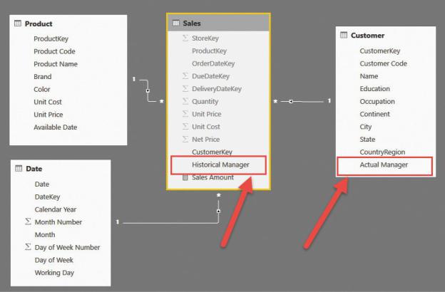
FIGURE 5-28 Denormalizing the historical manager in the fact table leads to a simple model.
Building the model is straightforward. You only need to compute, for each sale, the sales manager assigned to the customer’s country or region at the time of the sale. You can obtain this with a couple of merge operations—and, most importantly, without having to update the granularity of either the fact table or the dimension.
Regarding SCDs, here is a simple rule of thumb: If possible, try to isolate the slowly changing attribute (or set of attributes) and build a separate dimension for those attributes. You do not need to update the granularity. If the number of attributes is too large, then the best option is to go for the much more complex process of building a full SCD.
Conclusions
SCDs are not easy to manage. Yet, in many cases, it is important to use them because you want to track what happened in a relationship and attempt to predict what might happen in the future. The following are the important points to
remember from this chapter:
 What changes is not the dimension. It is a set of attributes of a dimension. Thus, the proper way of expressing the changing nature of your data is to understand what the slowly changing attributes are.
 You use historical attributes when analyzing the past. You use current attributes when projecting the current data to forecast the future.
 If you have a small set of slowly changing attributes, you can safely denormalize them in the fact table. If a dimension is needed for those attributes, you can build a historical dimension as a separate one.
 If the number of attributes is too large, you must follow the SCD pattern, knowing that the loading process will be much more complex and errorprone.
 If you build an SCD, you must move the granularity of both the fact table and the dimension to the version of the entity instead of the original entity.
 When you manage SCDs, most of the counting calculations must be adjusted to handle the new granularity, typically by using a distinct count instead of simple counts.