

author code that does not compute the totals in the right way. It is always good to double-check all the numbers before considering them correct.
 To optimize the code, precompute information whenever possible You should precompute the information about which dates are present in the snapshot by using a calculated column in the date table. This small change results in much better performance.
What you learned in this section applies to nearly all kinds of snapshots. You might need to handle the price of a stock, the temperature of an engine, or any kind of measurement. They all fall in the same category. Sometimes, you will need the value at the beginning of the period. Other times, it will be the value at the end. However, you will seldom be able to use a simple sum to aggregate values from the snapshot.
Understanding derived snapshots
A derived snapshot is a pre-aggregated table that contains a concise view of the values. Most of the time, snapshots are created for performance reasons. If you need to aggregate billions of rows every time you want to compute a number, then it might be better to precompute the value in a snapshot to reduce the computational effort of your model.
Often, this is a good idea, but you must carefully balance the pros and cons before choosing a snapshot for your model. Imagine, for example, that you must build a report that shows the number of customers for every month, dividing them into new customers and returning ones. You can leverage a precomputed table, like the one shown in Figure 6-7, which contains the three values you need for every month.
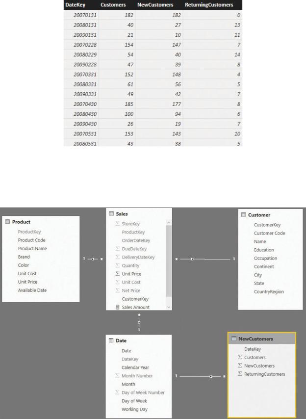
FIGURE 6-7 This table contains new and returning customers as a snapshot.
This pre-aggregated table, named NewCustomers, can be added to the model and joined through relationships with the Date table. This will enable you to build reports on top of it. Figure 6-8 shows the resulting model.
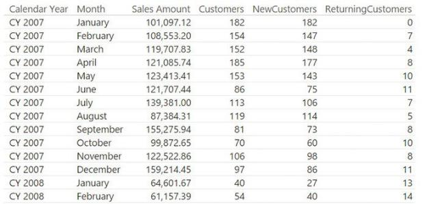
FIGURE 6-8 NewCustomers is a snapshot table linked in the model.
This snapshot contains only one row per month, for a total of 36 rows. When compared to the millions of rows in the fact table, it looks like a great deal. In fact, you can easily build a report that shows the sales amount along with the precomputed values, as shown in Figure 6-9.
FIGURE 6-9 A monthly report is very easy to generate with a snapshot.
From a performance point of view, this report is great because all the numbers are precomputed and available in a matter of milliseconds. Nevertheless, in a scenario like this, speed comes at a cost. In fact, the report has the following issues:
 You cannot generate subtotals As with the snapshot shown in the previous section, you cannot generate subtotals by aggregating with SUM. Worse, in this case, the numbers are all computed with distinct counts—meaning you cannot aggregate them by using LASTDATE or any other technique.
 You cannot slice by any other attribute Suppose you are interested in the same report, but limited to customers who bought some kind of product. In that case, the snapshot is of no help. The same applies to the date or any other attribute that goes deeper than the month.
In such a scenario, because you can obtain the same calculation by using a measure, the snapshot is not the best option. If you must handle tables that have less than a few hundred million rows, then making derived snapshots is not a good option. Calculations on the fly typically provide good performance and much more
flexibility.
With that said, there are scenarios in which you don’t want flexibility or need to avoid it. In those scenarios, snapshots play a very important role in the definition of the data model, even if they are derived snapshots. In the next section, we analyze one of these scenarios, the transition matrix.
Understanding the transition matrix
A transition matrix is a very useful modeling technique that makes extensive use of snapshots to create powerful analytical models. It is not an easy technique, but we think it is important that you understand at least the basic concepts of the transition matrix. It can be a useful tool for your modeling tool belt.
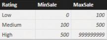
Suppose you assign a ranking to your customers based on how much they bought in a month. You have three categories of customers—low, medium, and high—and you have a Customer Rankings configuration table that you use to store the boundaries of each category, as shown in Figure 6-10.
FIGURE 6-10 The Customer Rankings configuration table for the rating of a customer.
Based on this configuration table, you can build a calculated table in the model that ranks each customer on a monthly basis, by using the following code:
Click here to view code image
CustomerRanked =
SELECTCOLUMNS (
ADDCOLUMNS (
SUMMARIZE ( Sales, 'Date'[Calendar Year], 'D
"Sales", [Sales Amount],
"Rating", CALCULATE (
VALUES ( 'Rating Configuration'[Rating]
FILTER (
'Ranking Configuration',
AND (
'Ranking Configuration'[MinSale]
'Ranking Configuration'[MaxSale]
)
)
),
"DateKey", CALCULATE ( MAX ( 'Date'[DateKey]
),
"CustomerKey", [CustomerKey], "DateKey", [DateKey], "Sales", [Sales],
"Rating", [Rating]
)
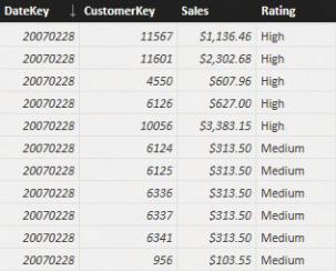
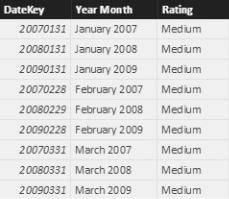
This query looks rather complex, but in reality, its result is simple. It produces a list of month, year, and customer keys. Then, based on the configuration table, it assigns to each customer a monthly rating. The resulting CustomerRanked table is shown in Figure 6-11.
FIGURE 6-11 The rating snapshot stores the ratings of customers on a monthly basis.
Depending on how much a customer buys, that customer may be rated differently in different months. Or, there may be several months when the customer has no rating at all. (This only means the customer did not buy anything in those months.) If you add the table to the model and build the proper set of relationships, you will obtain the data model shown in Figure 6-12. If, at this point, you think we are building a derived snapshot, you are right. CustomerRanked is a derived snapshot that precomputes a metric based on Sales, which actually stores the facts.
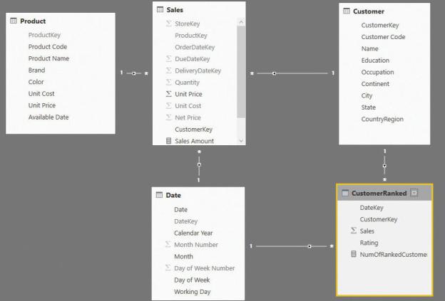
FIGURE 6-12 The snapshot, as always, looks like another fact table in the model.
You can use this table to build a simple report that shows the number of customers rated in different months and years. It is worth noting that this snapshot must be aggregated by using a distinct count, to consider each customer only once at the total level. The following formula is used to generate the measure found in the report shown in Figure 6-13:
Click here to view code image
NumOfRankedCustomers := CALCULATE (
DISTINCTCOUNT ( CustomerRanked[CustomerKey] )
)
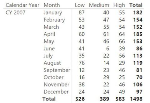
FIGURE 6-13 Using a snapshot to count the number of customers for a given rating is straightforward.
So far, we have built a snapshot table that looks very similar to the example in the previous section, which ended with a suggestion not to use a snapshot for that scenario. What is different here? The following are some important differences:
 The rating is assigned, depending on how much the customer spent, no matter what product was purchased. Because the definition of the rating is independent from the external selection, it makes sense to precompute it and to store it once and forever.
 Further slicing at the day level, for example, does not make much sense because the rating is assigned based on the sales of the whole month. Therefore, the very concept of month is included in the rating assigned.
Those considerations are already strong enough to make the snapshot a good solution. Nevertheless, there is a much stronger reason to do it. You can turn this snapshot into a transition matrix and perform much more advanced analyses.
A transition matrix aims to answer questions like, what is the evolution of the ranking of customers who were ranked medium in January 2007? The report required is like the one shown in Figure 6-14. It contains the customers who had a medium ranking in January 2007, and shows how their rankings changed over time.
FIGURE 6-14 The transition matrix provides very powerful insights in your customer analysis.
Figure 6-14 shows that in January 2007, 40 customers had a medium ranking. Of those customers, one was ranked high in April, one low in May, and one high in November. In 2009, four of those 40 customers had a low ranking in June. As you see, you set a filter for a given ranking in one month. This filter identifies a set of customers. You can then analyze how that set of customers behaved in other periods.
To build the transition matrix, you must perform the following two distinct operations:
1.Identify the customers who were ranked with a given ranking and date.
2.Check how they were ranked in different periods.
Let us start with the first operation. We want to isolate the customers with a given rating in one month. Because we want to use a slicer to fix the snapshot date and rating, we need a helper table to use as the filter. This point is important to understand. As an example, think about filtering the date of the snapshot (January 2007, in this example). If you use the Date table as a filter, then you use the same table that will be used also to show the evolution over time. In other words, if you use the Date table to filter January 2007, that filter will be effective on the entire model, making it impossible (or, rather, very hard) to build the report because you will not be able to see the evolution in, for example, February 2007.
Because you cannot use the Date table as a filter for the snapshot, the best option is to build a new table to serve as the source of the slicers. Such a table contains two columns: one with the different ratings and one with the months referenced by the fact table. You can build it using the following code:
Click here to view code image
SnapshotParameters = SELECTCOLUMNS (
ADDCOLUMNS ( SUMMARIZE (
CustomerRanked, 'Date'[Calendar Year], 'Date'[Month], CustomerRanked[Rating]
),
"DateKey", CALCULATE ( MAX ( 'Date'[DateKey]
),
"DateKey", [DateKey], "Year Month", FORMAT (
CALCULATE ( MAX ( 'Date'[Date] ) ), "mmmm YYYY"
),
"Rating", [Rating]
)
Figure 6-15 shows the resulting table (SnapshotParameters).
FIGURE 6-15 The SnapshotParameters table contains three columns.
The table contains both the date key (as an integer) and the year month (as a string). You can put the string in a slicer and grab the corresponding key that will be useful when moving the filter to the snapshot table.
This table should not be related to any other table in the model. It is merely a helper table, used as the source of two slicers: one for the snapshot date and one for the snapshot rating. The data model is now in place. You can select a starting
point for the ranking and put the years and months in the rows of a matrix. The following DAX code will compute the desired number—that is the number of customers who had a given rating in the selection from the slicer and a different rating in different periods:
Click here to view code image
Transition Matrix = CALCULATE (
DISTINCTCOUNT ( CustomerRanked[CustomerKey] ), CALCULATETABLE(
VALUES ( CustomerRanked[CustomerKey] ), INTERSECT (
ALL ( CustomerRanked[Rating] ), VALUES ( SnapshotParameters[Rating] )
), INTERSECT (
ALL ( CustomerRanked[DateKey] ), VALUES ( SnapshotParameters[DateKey] )
),
ALL ( CustomerRanked[RatingSort] ), ALL ( 'Date' )
)
)
This code is not easy to understand at first sight, but we suggest you to spend some time studying it carefully. It expresses so much power in so few lines that you will probably grasp some new ideas from understanding it.
The core of the code is the CALCULATETABLE function, which uses two INTERSECT calls. INTERSECT is used to apply the selection from SnapshotParameters (the table used for the slicers) as a filter of CustomerRanked. There are two INTERSECT calls: one for the date, one for the ranking. When this filter is in place, CALCULATETABLE returns the keys of the customers who were ranked with the given rating at the given date. Thus, the outer CALCULATE will compute the number of customers ranked in different periods, but limit the count to only the ones selected by CALCULATETABLE. The resulting report is the one already shown in Figure 6-14.
From a modeling point of view, it is interesting that you need a snapshot table to perform this kind of analysis. In fact, in this case, the snapshot is used to determine the set of customers who had a specific rating in a given month. This