

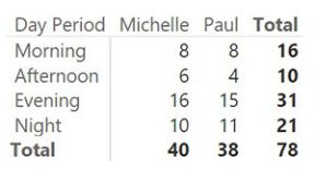
As mentioned, one of the big advantages of splitting date and time is to be able to analyze the time as a dimension by itself, unrelated to dates. If you want to analyze the shifts for which a worker is mostly employed, you can build a simple matrix like the one shown in Figure 7-11. In this figure, we used a version of the time dimension that includes, as indicated earlier in the chapter, day periods that contain only 24 rows. This is because we are interested in the hours only.
FIGURE 7-11 This figure shows an analysis of time periods that are unrelated to dates.
At this point, you can compute the hourly rate (which will probably require some sort of configuration table) and perform a much finer analysis on the model. Nevertheless, in this demonstration, we were mainly focused on finding the correct granularity. We can stop analyzing this example here.
The important part of this demo is that, by finding the correct granularity, we moved from a very complex DAX expression to a much simpler one. At the same time, we increased the analytical power of our data model. We are perfectly aware of how many times we repeat the same concept. But this way, you can see how important it is to perform a deep analysis of the granularity needed by your model, depending on the kind of analysis you want to perform.
It does not matter how the original data is shaped. As a modeler, you must continue massaging your data until it reaches the shape needed by your model. Once it reaches the optimal format, all the numbers come out quickly and easily.
Modeling working shifts and time shifting
In the previous example, we analyzed a scenario where the working shifts were easy to get. In fact, the time at which the worker started the shift was part of the model. This is a very generic scenario, and it is probably more complex than what the average data analyst needs to cover.
In fact, having a fixed number of shifts during the day is a more common scenario. For example, if a worker normally works eight hours a day, there can be
three different shifts that are alternately assigned to a worker during the month. It is very likely that one of these shifts will cross into the next day, and this makes the scenario look very similar to the previous one.
Another example of time shifting appears in a scenario where you want to analyze the number of people who are watching a given television channel, which is commonly used to understand the composition of the audience of a show. For example, suppose a show starts at 11:30 p.m., and it is two hours long, meaning it will end the next day. Nevertheless, you want it to be included in the previous day. And what about a show that starts at half past midnight? Do you want to consider it in competition with the previous show that started one hour earlier? Most likely, the answer is yes, because no matter when the two shows started, they were playing at the same time. It is likely an individual chose either one or the other.
There is an interesting solution to both these scenarios that requires you to broaden your definition of time. In the case of working shifts, the key is to ignore time completely. Instead of storing in the fact table the starting time, you can simply store the shift number, and then perform the analysis using the shift number only. If you need to consider time in your analysis, then the best option is to lower the granularity and use the previous solution. However, in most cases, we solved the model by simply removing the concept of time from the model.
The audience analysis scenario is somewhat different, and the solution, although strange, is very simple. You might want to consider the events happening right after midnight as belonging to the previous day so that when you analyze the audience of one day, you consider in the total what happened after midnight. To do so, you can easily implement a time-shifting algorithm. For example, instead of considering midnight as the beginning of the day, you can make the day start at 02:00 a.m. You can then add two more hours to the standard time so that the time ranges from 02:00 to 26:00 instead of going from 00:00 to 24:00. It is worth noting that, for this specific example, using the 24-hour format (26, to be precise) works much better than using a.m./p.m.
Figure 7-12 shows a typical report that uses this time-shifting technique. Note that the custom period starts at 02:00 and ends at 25:59. The total is still 24 hours, but by shifting time in this way, when you analyze the audience of one day, you also include the first two hours of the next day.
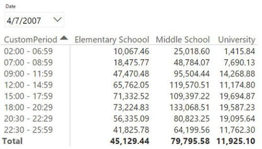
FIGURE 7-12 By using the time-shifting technique, the day starts at 02:00 instead of starting at midnight.
Obviously, when loading the data model for such a scenario, you will need to perform a transformation. However, you will not be able to use DateTime columns because there is no such time as 25:00 in a normal date/time.
Analyzing active events
As you have seen, this chapter mainly covers fact tables with the concept of duration. Whenever you perform an analysis of these kinds of events, one interesting model is one that analyzes how many events were active in a given period. An event is considered active if it is started and not yet finished. There are many different kinds of these events, including orders in a sales model. An order is received, it is processed, and then it is shipped. In the period between the date of receipt and the date of shipment, the order is active. (Of course, in performing this analysis, you can go further and think that between shipment and delivery to the recipient, the order is still active, but in a different status.)
For the sake of simplicity, we are not going to perform a complex analysis of those different statuses. Here, we are mainly interested in discovering how you can build a data model to perform an analysis of active events. You can use such a model in different scenarios, like insurance policies (which have a start and end date), insurance claims, orders growing plants, or building items with a type of machinery. In all these cases, you record as a fact the event (such as the plants grown, the order placed, or the full event). However, the event itself has two or
more dates identifying the process that has been executed to bring the event to its conclusion.
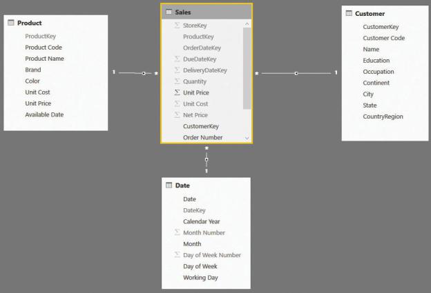
Before starting to solve the scenario, let us look at the first consideration you must account for when analyzing orders. The data model we used through most of this book stores sales at the granularity of the product, date, and customer level. Thus, if a single order contains 10 different products, it is represented with 10 different lines in the Sales table. Such a model is shown in Figure 7-13.
FIGURE 7-13 The fact table in this model stores individual sales.
If you want to count the number of orders in this model, you will need to perform a distinct count of the Order Number column in Sales, because a given order number will be repeated for multiple rows. Moreover, it is very likely that, if an order was shipped in multiple packages, different lines in the same order might have different delivery dates. So, if you are interested in analyzing the open orders, the granularity of the model is wrong. In fact, the order as a whole is to be considered delivered only when all its products have been delivered. You can compute the date of delivery of the last product in the order with some complex DAX code, but in this case, it is much easier to generate a new fact table containing only the orders. This will result in a lower granularity, and it will
reduce the number of rows. Reducing the number of rows has the benefit of speeding up the calculation and avoiding the need to perform distinct counts.
The first step is to build an Orders table, which you can do with SQL, or, as we are doing in the example, with a simple calculated table that uses the following code:
Click here to view code image
Orders = SUMMARIZECOLUMNS (
Sales[Order Number],
Sales[CustomerKey],
"OrderDateKey", MIN ( Sales[OrderDateKey] ), "DeliveryDateKey", MAX ( Sales[DeliveryDateKey]
)
This new table has fewer rows and fewer columns. It also already contains the first step of our calculation, which is the determination of the effective date of delivery, by taking into account the last delivery date of the order as a whole. The resulting data model, once the necessary relationships are created, is shown in Figure 7-14.
FIGURE 7-14 The new data model contains two fact tables at different granularities.
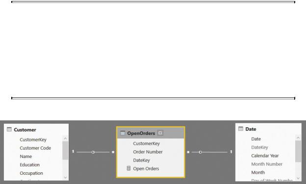
You can see that the Orders table has no relationships with Product. It is worth noting that you can also model such a scenario using a standard header/detail table, with Orders as the header and Sales as the detail. In such a case, you should take into account all the considerations we already made in Chapter 2, “Using header/detail tables.” In this section, we ignore the header/detail relationship because we are mainly interested in using the Orders table only. Thus, we will use a simplified model, as shown in Figure 7-15. (Note that in the companion file, the
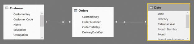
Sales table is still present, because Orders depends on it. However, we will focus on these three tables only.)
FIGURE 7-15 This figure shows the simplified model we use for this demo.
After the model is in place, you can easily build a DAX measure that computes the number of open orders by using the following code:
Click here to view code image
OpenOrders := CALCULATE (
COUNTROWS ( Orders ), FILTER (
ALL ( Orders[OrderDateKey] ), Orders[OrderDateKey] <= MIN ( 'Date'[DateKey
), FILTER (
ALL ( Orders[DeliveryDateKey] ), Orders[DeliveryDateKey] > MAX ( 'Date'[DateK
),
ALL ( 'Date' )
)
The code itself is not complex. The important point is that because there is a relationship between Orders and Date that is based on OrderDateKey, you must remove its effects by using ALL on the Date table. Forgetting to do so will return a wrong number—basically the same number as the orders placed. The measure itself works just fine, as you can see in Figure 7-16, which shows both the number of orders received and the number of open orders.
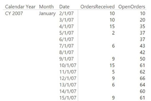
FIGURE 7-16 The report shows the number of orders received and the number of open orders.
To check the measure, it would be useful to show both the orders received and the orders shipped in the same report. This can be easily accomplished by using the technique you learned in Chapter 3, “Using multiple fact tables,” which is adding a new relationship between Orders and Date. This time, the relationship will be based on the delivery date and kept inactive to avoid model ambiguity. Using this new relationship, you can build the OrdersDelivered measure in the following way:
Click here to view code image
OrdersDelivered := CALCULATE (
COUNTROWS ( Orders ),
USERELATIONSHIP ( Orders[DeliveryDateKey], 'Date
)
At this point, the report looks easier to read and check, as shown in Figure 7- 17.
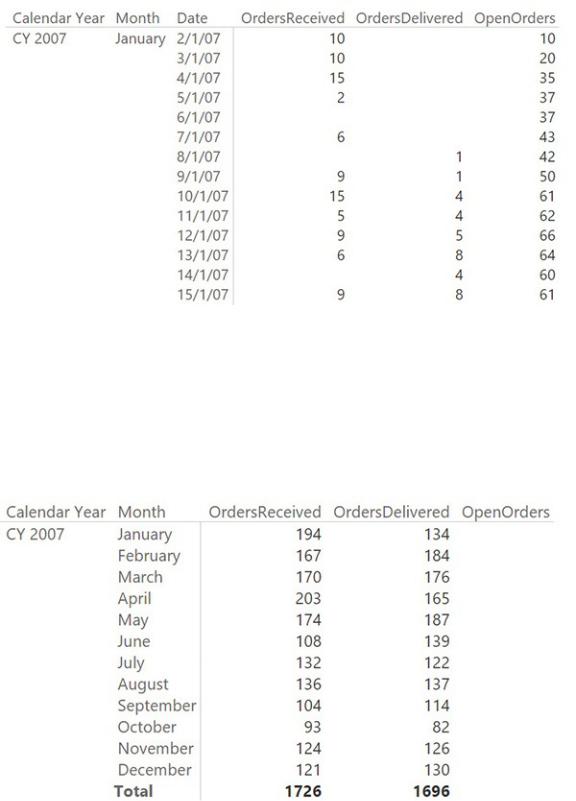
FIGURE 7-17 Adding the OrdersDelivered measure makes the report easier to understand.
This model provides the correct answers at the day level. However, at the month level (or on any other level above the day level), it suffers from a serious drawback. In fact, if you remove the date from the report and leave only the month, the result is surprising: The OpenOrders measure always shows a blank, as shown in Figure 7-18.
FIGURE 7-18 At the month level, the measure produces the wrong (blank)
results.
The issue is that no orders lasted for more than one month, and this measure returns the number of orders received before the first day of the selected period and delivered after the end of that period (in this case, a month). Depending on your needs, you must update the measure to show the value of open orders at the end of the period, or the average value of open orders during the period. For example, the version that computes the open orders at the end of the period is easily produced with the following code, where we simply added a filter for LASTDATE around the original formula.
Click here to view code image
OpenOrders := CALCULATE (
CALCULATE (
COUNTROWS ( Orders ), FILTER (
ALL ( Orders[OrderDateKey] ), Orders[OrderDateKey] <= MIN ( 'Date'[Dat
), FILTER (
ALL ( Orders[DeliveryDateKey] ), Orders[DeliveryDateKey] > MAX ( 'Date'[D
),
ALL ( 'Date' )
),
LASTDATE ( 'Date'[Date] )
)
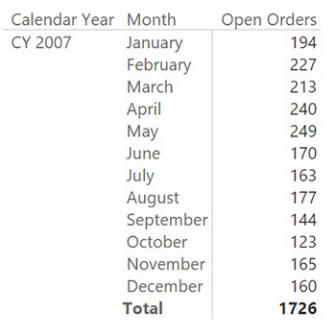
With this new formula, the result at the month level is as desired, as shown in Figure 7-19.
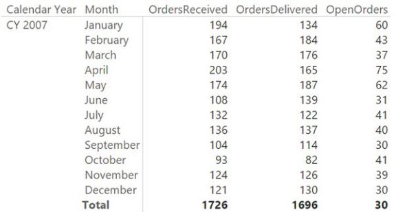
FIGURE 7-19 This report shows, at the month level, the orders that were open on the last day of the month.
This model works just fine, but in older versions of the engine (that is, in Excel 2013 and in SQL Server Analysis Services 2012 and 2014), it might result in very bad performance. The new engine in Power BI and Excel 2016 is much faster, but this measure is still not a top performer. Explaining the exact reason for this poor performance is beyond the scope of this book, but in a few words, we can say that the problem is in the fact that the condition of filtering does not make use of relationships. Instead, it forces the engine to evaluate the two conditions in its slower part, known as the formula engine. On the other hand, if you build the model in such a way that it relies only on relationships, then the formula will be faster.
To obtain this result, you must change the data model, modifying the meaning of the facts in the fact table. Instead of storing the duration of the order by using the start and end date, you can store a simpler fact that says, “this order, on this date, was still open.” Such a fact table needs to contain only two columns: Order Number and DateKey. In our model, we moved a bit further, and we also added the customer key so that we could slice the orders by customer, too. The new fact table can be obtained through the following DAX code:
Click here to view code image
OpenOrders =
SELECTCOLUMNS (
GENERATE ( Orders,
VAR CurrentOrderDateKey = Orders[OrderDateKe VAR CurrentDeliverDateKey = Orders[DeliveryD RETURN
FILTER (
ALLNOBLANKROW ( 'Date'[DateKey] ), AND (
'Date'[DateKey] >= CurrentOrderD 'Date'[DateKey] < CurrentDeliver
)
)
),
"CustomerKey", [CustomerKey], "Order Number", [Order Number], "DateKey", [DateKey]
)
 Note
Note
Although we provide the DAX code for the table, it is more likely that you can produce such data using the Query Editor or a SQL view. Because DAX is more concise than SQL and M, we prefer to publish DAX code, but please do not assume that this is the best solution in terms of performance. The focus of this book is on the data model itself, not on performance considerations about how to build it.
You can see the new data model in Figure 7-20.
FIGURE 7-20 The new Open Orders table only contains an order when it is open.
In this new data model, the whole logic of when an order is open is stored in
the table. Because of this, the resulting code is much simpler. In fact, the Open Orders measure is the following single line of DAX:
Click here to view code image
Open Orders := DISTINCTCOUNT ( OpenOrders[Order
Number] )
You still need to use a distinct count because the order might appear multiple times, but the whole logic is moved into the table. The biggest advantage of this measure is that it only uses the fast engine of DAX, and it makes much better use of the cache system of the engine. The OpenOrders table is larger than the original fact table, but with simpler data, it is likely to be faster. In this case, as in the case of the previous model, the aggregation at the month level produces unwanted results. In fact, at the month level, the previous model returned orders that were open at the beginning and not closed until the end, resulting in blank values. In this model, on the other hand, the result at the month level is the total number of orders that were open on at least one day during the month, as shown in Figure 7-21.
FIGURE 7-21 This new model returns, at the month level, the orders that were open sometime during the month.
You can easily change this to the average number of open orders or to the open orders at the end of the month by using the following two formulas:
Click here to view code image
Open Orders EOM := CALCULATE ( [Open Orders],
LASTDATE ( ( 'Date'[Date] ) ) )
Open Orders AVG := AVERAGEX ( VALUES (
'Date'[DateKey] ), [Open Orders] )
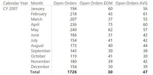
You can see an example of the resulting report in Figure 7-22.
FIGURE 7-22 This report shows the total, average, and end-of-month number of open orders.
It is worth noting that computing open orders is a very CPU-intensive operation. It might result in slow reports if you have to handle several million orders. In such a case, you might also think about moving more computational logic into the table, removing it from the DAX code. A good example might be that of pre-aggregating the values at the day level by creating a fact table that contains the date and the number of open orders. In performing this operation, you obtain a very simple (and small) fact table that has all the necessary values already precomputed, and the code becomes even easier to author.
You can create a pre-aggregated table with the following code:
Click here to view code image
Aggregated Open Orders = FILTER (
ADDCOLUMNS (
DISTINCT ( 'Date'[DateKey] ),
"OpenOrders", [Open Orders]
),
[Open Orders] > 0
)
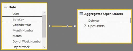
The resulting table is tiny because it has the same granularity as the date table. Thus, it contains a few thousand rows. This model is the simplest of the set of models that we analyzed for this scenario because, having lost the order number and the customer key, the table has a single relationship with the date. You can see this in Figure 7-23. (Again, note that the companion file contains more tables. This is because it contains the whole model, as will be explained later in this section.)
FIGURE 7-23 Pre-aggregating open orders produces an amazingly simple data model.
In this model, the number of open orders is computed in the simplest way, because you can easily aggregate the OpenOrders column by SUM.
At this point, the careful reader might object that we went several steps back in our learning of data modeling. In fact, at the very beginning of the book, we said that working with a single table where everything is already precomputed is a way to limit your analytical power. This is because if a value is not present in the table, then you lose the capability to slice at a deeper level or to compute new values. Moreover, in Chapter 6, “Using snapshots,” we said that this preaggregation in snapshots is seldom useful—and now we are snapshotting open orders to improve the performance of a query!
To some extent, these criticisms are correct, but we urge you to think more about this model. The source data is still available. What we did this time does not reduce the analytical power. Instead, seeking top performance, we built a snapshot table using DAX that includes most of the computational logic. In this way, heavy-to-compute numbers like the value of open orders can be gathered from the pre-aggregated table while, at the same time, more lightweight values