

Chapter 2. Using header/detail tables
Now that you have a basic understanding of the concepts of data modeling, we can start discussing the first of many scenarios, which is the use of header/detail tables. This scenario happens very frequently. By themselves, header/detail tables are not a complex model to use. Nevertheless, this scenario hides some complexities whenever you want to mix reports that aggregate numbers at the two different levels.
Examples of header/detail models include invoices with their lines or orders with their lines. Bills of materials are also typically modeled as header/detail tables. Another example would be if you need to model teams of people. In this case, the two different levels would be the team and the people.
Header/detail tables are not to be confused with standard hierarchies of dimensions. Think, for example, about the natural hierarchy of a dimension that is created when you have products, subcategories, and categories. Although there are three levels of data, this is not a header/detail pattern. The header/detail structure is generated by some sort of hierarchical structure on top of your events—that is, on top of your fact tables. Both an order and its lines are facts, even if they are at different granularities, whereas products, categories, and subcategories are all dimensions. To state it in a more formal way, header/detail tables appear whenever you have some sort of relationship between two fact tables.
Introducing header/detail
As an example, we created a header/detail scenario for the Contoso database. You can see its data model in Figure 2-1.
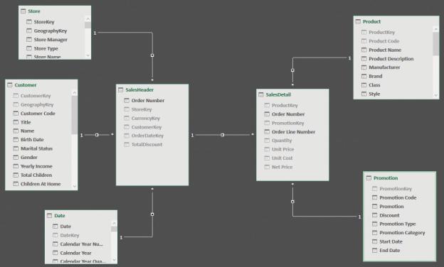
FIGURE 2-1 SalesHeader and SalesDetail comprise a header/detail scenario.
Based on the previous chapter, you might recognize this model as a slightly modified star schema. In fact, if you look at SalesHeader or SalesDetail individually, with their respective related tables, they are star schemas. However, when you combine them, the star shape is lost because of the relationship linking SalesHeader and SalesDetail. This relationship breaks the star schema rules because both the header and detail tables are fact tables. At the same time, the header table acts as a dimension for the detail.
At this point, you might argue that if we consider SalesHeader a dimension instead of a fact table, then we have a snowflake schema. Moreover, if we denormalize all columns from Date, Customer, and Store in SalesHeader, we can re-create a perfect star schema. However, there are two points that prevent us from performing this operation. First, SalesHeader contains a TotalDiscount metric. Most likely, you will aggregate values of TotalDiscount by customer. The presence of a metric is an indicator that the table is more likely to be a fact table than a dimension. The second, and much more important, consideration is that it would be a modeling error to mix Customer, Date, and Store in the same dimension by denormalizing their attributes in SalesOrderHeader. This is because these three dimensions make perfect sense as business assets of Contoso, whereas if you mix all their attributes into a single dimension to rebuild a star schema, the
model would become much more complex to browse.
As you will learn later in this chapter, for such a schema, the correct solution is not to mix the dimensions linked to the header into a single, new dimension, even if it looks like a nice idea. Instead, the best choice is to flatten the header into the detail table, increasing the granularity. There will be more on this later in the chapter.
Aggregating values from the header
Apart from aesthetic issues (it is not a perfect star schema), with header/detail models, you need to worry about performance and, most importantly, how to perform the calculations at the right granularity. Let us analyze the scenario in more detail.
You can compute any measure at the detail level (such as the sum of quantity and sum of sales amount), and everything works fine. The problems start as soon as you try to aggregate values from the header table. You might create a measure that computes the discount value, stored in the header table, with the following code:
Click here to view code image
DiscountValue := SUM ( SalesHeader[TotalDiscount] )
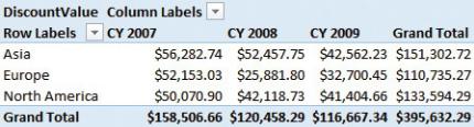
The discount is stored in the header because it is computed over the whole order at the time of the sale. In other words, the discount is granted over the entire order instead of being applied to each line. For this reason, it is saved in the header table. The DiscountValue measure works correctly as long as you slice it with any attribute of a dimension that is directly linked to SalesHeader. In fact, the PivotTable shown in Figure 2-2 works just fine. It slices the discount by continent (the column in Store, linked to SalesHeader) and year (the column in Date, again linked to SalesHeader).
FIGURE 2-2 You can slice discount by year and continent, producing this PivotTable.
However, as soon as you use one of the attributes of any dimension that is not
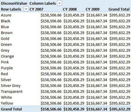
directly related to SalesHeader, the measure stops working. If, for example, you slice by the color of a product, then the result is what is shown in Figure 2-3. The filter on the year works fine, exactly as it did in the previous PivotTable.
However, the filter on the color repeats the same value for each row. In some sense, the number reported is correct, because the discount is saved in the header table, which is not related to any product. Product is related to the detail table, and a discount saved in the header is not expected to be filtered by product.
FIGURE 2-3 If you slice the discount by a product color, the same number is repeated on each row.
A very similar issue would occur for any other value stored in the header table. For example, think about the freight cost. The cost of the shipment of an order is not related to the individual products in the order. Instead, the cost is a global cost for the shipment, and again, it is not related to the detail table.
In some scenarios, this behavior is correct. Users know that some measures cannot simply be sliced by all the dimensions, as it would compute inaccurate values. Nevertheless, in this specific case, we want to compute the average discount percentage for each product and then deduct this information from the header table. This is a bit more complicated than one might imagine. This is due to the data model.
If you are using Power BI or Analysis Services Tabular 2016 or later, then you
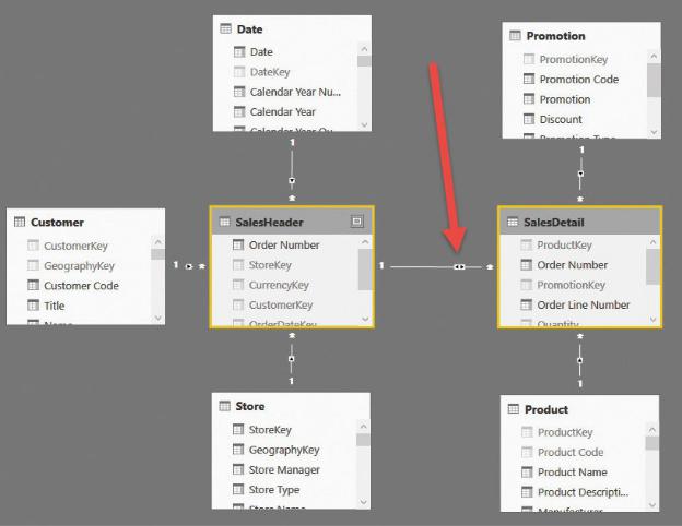
have access to bidirectional filtering, meaning you can instruct the model to propagate the filter on SalesDetail to SalesHeader. In this way, when you filter a product (or a product color), the filter will be active on both SalesHeader and SalesDetail, showing only the orders containing a product of the given color. Figure 2-4 shows the model with bidirectional filtering activated for the relationship between SalesHeader and SalesDetail.
FIGURE 2-4 If bidirectional filtering is available, you can let the filter propagate in both directions of the relationship.
If you work with Excel, then bidirectional filtering is not an option at the datamodel level. However, you can obtain the same result by modifying the measure using the bidirectional pattern with the following code. (We’ll talk about this in more detail in Chapter 8, “Many-to-many relationships.”)
Click here to view code image
DiscountValue :=
CALCULATE (
SUM ( SalesHeader[TotalDiscount] ),
CROSSFILTER ( SalesDetail[Order Number], SalesHe
)
It appears that a small change in the data model (enabling bidirectional filtering on the relationship) or in the formula (using the bidirectional pattern) solves the issue. Unfortunately, however, neither of these measures compute a meaningful value. To be precise, they compute a meaningful value, but it has a meaning that is totally different from what you would expect.
Both techniques move the filter from SalesDetail to SalesHeader, but they then aggregate the total discount for all the orders that contain the selected products. The issue is evident if you create a report that slices by brand (which is an attribute of Product, indirectly related to SalesHeader) and by year (which is an attribute of Date, directly related to SalesHeader). Figure 2-5 shows an example of this, in which the sum of the highlighted cells is much greater than the grand total.
FIGURE 2-5 In this PivotTable, the sum of the highlighted cells is $458,265.70, which is greater than the grand total.
The issue is that, for each brand, you are summing the total discount of the orders that contain at least one product of that brand. When an order contains products of different brands, its discount is counted once for each of the brands. Thus, the individual numbers do not sum at the grand total. At the grand total, you get the correct sum of discounts, whereas for each brand, you obtain a number that is greater than what is expected.

 Info
Info
This is an example of a wrong calculation that is not so easy to spot. Before we proceed, let us explain exactly what is happening. Imagine you have two orders: one with apples and oranges, and one with apples and peaches. When you slice by product using bidirectional filtering, the filter will make both orders visible on the row with apples, so the total discount will be the sum of the two orders. When you slice by oranges or peaches, only one order will be visible. Thus, if the two orders have a discount of 10 and 20, respectively, you will see three lines: apples 30, oranges 10, and peaches 20. For the grand total, you will see 30, which is the total of the two orders.
It is important to note that by itself, the formula is not wrong. In the beginning, before you are used to recognizing issues in the data model, you tend to expect DAX to compute a correct number, and if the number is wrong, you might think there is an error in the formula. This is often the case, but not always. In scenarios like this one, the problem is not in the code, but in the model. The issue here is that DAX computes exactly what you are asking for, but what you are asking for is not what you want.
Changing the data model by simply updating the relationship is not the right way to go. We need to find a different path to the solution. Because the discount is stored in the header table as a total value, you can only aggregate that value, and this is the real source of the error. What you are missing is a column that contains the discount for the individual line of the order so that when you slice by one of the attributes of a product, it returns a correct value. This problem is again about granularity. If you want to be able to slice by product, you need the discount to be at the order-detail granularity. Right now, the discount is at the order header granularity, which is wrong for the calculation you are trying to build.
At the risk of being pedantic, let us highlight an important point: You do not need the discount value at the product granularity, but at the SalesDetail granularity. The two granularities might be different— for example, in case you have two rows in the detail table that belong to the same order and have the same product ID. How can you obtain such a result? It is easier than you might think, once you recognize the problem. In fact, you can compute a column in SalesHeader that stores the discount as a percentage instead of an absolute value. To perform this, you need to divide the total discount by the total of the order. Because the total of the order is not stored in the SalesHeader table in our model,
you can compute it on the fly by iterating over the related detail table. You can see this in the following formula for a calculated column in SalesHeader:
Click here to view code image
SalesHeader[DiscountPct] = DIVIDE (
SalesHeader[TotalDiscount], SUMX (
RELATEDTABLE ( SalesDetail ), SalesDetail[Unit Price] * SalesDetail[Quanti
)
)
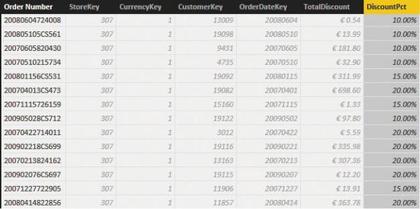
Figure 2-6 shows the result, with the SalesHeader table with the new column formatted as a percentage to make its meaning easy to understand.
FIGURE 2-6 The DiscountPct column computes the discount percentage of the order.
Once you have this column, you know that each of the individual lines of the same order has the same discount percentage. Thus, you can compute the discount amount at the individual line level by iterating over each row of the SalesDetail table. You can then compute the discount of that line by multiplying the header discount percentage by the current sales amount. For example, the following code replaces the previous version of the DiscountValue measure:
Click here to view code image
[DiscountValueCorrect] = SUMX (
SalesDetail,
RELATED ( SalesHeader[DiscountPct] ) * SalesDeta
)
It is also worth noting that this formula no longer needs the relationship between SalesHeader and SalesDetail to be bidirectional. In the demo file, we left it bidirectional because we wanted to show both
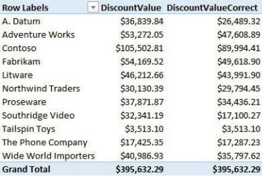
values together. In fact, in Figure 2-7, you can see the two measures side by side in a PivotTable. You will also see that DiscountValueCorrect reports a slightly lower number, which sums correctly at the grand-total level.
FIGURE 2-7 Having the two measures side by side shows the difference between them. Moreover, the correct value produces a sum that is identical to the grand total, as expected.
Another option, with a simpler calculation, is to create a calculated column in SalesDetail that contains the following expression, which is the discount value for the individual row that is precomputed in SalesDetail:
Click here to view code image
SalesDetail[LineDiscount] =
RELATED ( SalesHeader[DiscountPct] ) *
SalesDetail[Unit Price] *
SalesDetail[Quantity]
In this case, you can easily compute the discount value by summing the LineDiscount column, which already contains the correct discount allocated at the
individual row level.
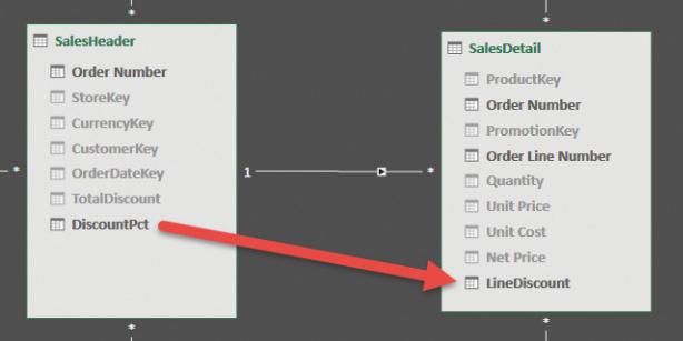
This approach is useful because it shows more clearly what we did. We changed the data model by denormalizing the discount from the SalesHeader table into the SalesDetail table. Figure 2-8 (which presents the diagram view) shows the two fact tables after we added the LineDiscount calculated column. SalesHeader no longer contains any value that is directly aggregated in a measure. The only metrics in the SalesHeader table are TotalDiscount and DiscountPct, which are used to compute LineDiscount in the SalesDetail table. These two columns should be hidden because they are not useful for analysis unless you want to use DiscountPct to slice your data. In that case, it makes sense to leave it visible.
FIGURE 2-8 The DiscountPct and TotalDiscount columns are used to compute LineDiscount.
Let us now draw some conclusions about this model. Think about this carefully. Now that the metric that was present in SalesHeader is denormalized in SalesDetail, you can think of SalesHeader as being a dimension. Because it is a dimension that has relationships with other dimensions, we have essentially transformed the model into a snowflake, which is a model where dimensions are linked to the fact table through other dimensions. Snowflakes are not the perfect choice for performance and analysis, but they work just fine and are valid from a modeling point of view. In this case, a snowflake makes perfect sense because the different dimensions involved in the relationships are, one by one, operational assets of the business. Thus, even if it is not very evident in this example, we