

Appendix A. Data modeling 101
The goal of this appendix is to explain the data-modeling concepts that are used throughout the book and that are often discussed in articles, blog posts, and books. It is not an appendix to read from the beginning to the end. Instead, you can take a quick look at this appendix if, while reading the book, you find a term or a concept that is not clear or you want to refresh your memory. Thus, the appendix does not have a real flow. Each topic is treated in its own self-contained section. Moreover, we do not want this to be a complex appendix. We provide only the basic information about the topics. An in-depth discussion of them is beyond the scope of this book.
Tables
A table is a container that holds information. Tables are divided into rows and columns. Each row contains information about an individual entity, whereas each cell in a row contains the smallest piece of information represented in a database. For example, a Customer table might contain information about all your customers. One row contains all the information about one customer, and one column might contain the name or the address of all the customers. A cell might contain the address for one customer.
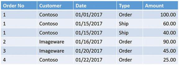
When building your model, you must think in these terms to avoid some common pitfalls that can make the analysis of your model a nightmare. Imagine, for example, that you decide to store information about an order in two rows of the same table. In one row, you store the amount ordered, along with its order date. In the other row, you store the amount shipped, again with its shipment date. By doing so, you split one entity (the order) into two rows of the same table. An example is shown in Figure A-1.
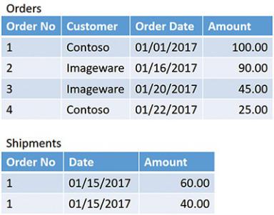
Figure A-1 In this table, information about a single order is divided into multiple rows.
This makes the table much more complex. Computing even a simple value like the order amount becomes more complex because a single column (Amount) contains different kinds of information. You cannot simply sum the amount; you always need to apply a filter. The problem with this model is that you have not designed it the right way. Because the individual order information is split into several rows, it is difficult to perform any kind of calculation. For example, computing the percentage of goods already shipped for every customer becomes a complex operation because you need to build code to do the following:
1.Iterate over each order number.
2.Aggregate the amount ordered (if it is in multiple lines), filtering only the rows in which the Type column equals Order.
3.Aggregate the amount shipped, this time filtering only the rows in which Type equals Ship.
4.Compute the percentage.
In the previous example, the error is that if an order is an entity in your model, then it needs to have its own table where all the values can be aggregated in a simple way. If you also need to track individual transactions for shipments, then you can build a Shipments table that contains only shipments. Figure A-2 shows you the correct model for this dataset.
Figure A-2 The correct representation of orders and shipments requires two
tables.
In this example, we only track shipments. However, you might have a more generic table that tracks the transactions of the order (orders, shipments, and returns). In that case, it is fine to store both types of transactions in the same table by tagging them with an attribute that identifies the type of operation. It is also fine to store different types of the same entity (transactions) in the same table. However, it is not good to store different entities (orders and transactions) in the same table.
Data types
When you design a model, each column has a data type. The data type is the type of content in the column. The data type can be integer, string, currency, floating point, and so on. There are many data types that you can choose from. The data type of a column is important because it affects its usability, the functions you can use on it, and the formatting options. In fact, the data type of a column is the format used internally by the engine to store the information. In contrast, the format string is only pertinent to how the UI represents the information in a human-readable form.
Suppose you have a column that should contain the quantity shipped. In that case, it is likely that an integer is a good data type for it. However, in a column that needs to store sales amounts, an integer is no longer a good option because you will need to store decimal points, too. In such a case, currency is the right data type to use.
When using plain Excel, each cell can contain values of any data type. When using the tabular data model, however, the data type is defined at the column level. This means all the rows in your table will need to store the same data type in that column. You cannot have mixed data types for one column in a table.
Relationships
When your model contains multiple entities, as is generally the case, you store information in multiple tables and link them through relationships. In a tabular model, a relationship always links two tables, and it is based on a single column.
The most common representation of a relationship is an arrow that starts from the source table and goes to the target table, as shown in Figure A-3.

Figure A-3 In this model, there are four tables that are linked through relationships.
When you define a relationship, there is always a one side and a many side. In the sample model, for each product, there are many sales, and for each sale there is exactly one product. Thus, the Product table is on the one side, whereas Sales is on the many side. The arrow always goes from the many side to the one side.
In different versions of Power Pivot for Excel and in Power BI, the user interface uses different visualizations for relationships. However, in the latest versions of both Excel and Power BI, the engine draws a line that tags the ends of the line with a 1 (one) or * (star) to identify the one or the many side of the relationship. In Power BI Desktop, you also have the option of creating one-to-one relationships. A one-to-one relationship is always bidirectional because for each row of a table, there can be only zero or one rows in the other table. Thus, in this special case, there is no many side of the relationship.
Filtering and cross-filtering
When you browse your model through a PivotTable or by using Power BI, filtering is very important. In fact, it is the foundation of most—if not all— calculations in a report. When using the DAX language, the rule is very simple: The filter always moves from the one side of a relationship to the many side. In the user interface, this is represented by an arrow in the middle of the relationship
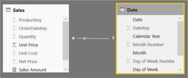
that shows how the filter propagates through the relationship, as shown in Figure A-4.
Figure A-4 The small arrow inside the line of the relationship represents the direction of the filter.
Thus, whenever you filter Date, you filter Sales, too. This is why, in a PivotTable, you can easily slice the sales amount by the calendar year: a filter on Date directly translates to a filter on Sales. The opposite direction, on the other hand, does not work by default. A filter on Sales will not propagate to Date unless you instruct the data model to do so. Figure A-5 shows you a graphical representation of how the filter is propagated by default.
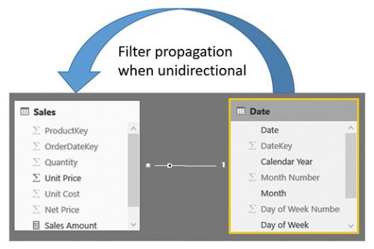
Figure A-5 The large arrow indicates how the filter is being propagated when unidirectional filtering is on.
You can change the direction of the filter propagation (known as cross-filter direction) by modifying the setting of the relationship. In Power BI, for example, this is done by double-clicking on the relationship itself. This opens the Edit Relationship dialog box, shown in Figure A-6.
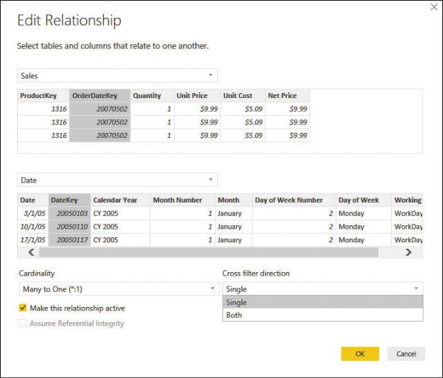
Figure A-6 The Edit Relationship dialog box lets you modify the cross-filter direction.
By default, the cross-filter direction is set to Single—that is, from one to many. If needed, you can change it to Both so that the filter also propagates from the many side to the one side. Figure A-7 shows a graphical representation of how the filter propagates when you set it to be bidirectional.
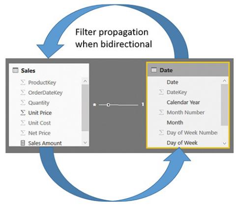
Figure A-7 When in bidirectional mode, the filter propagates both ways.
This feature is not available in Power Pivot for Excel 2016. If you need to activate bidirectional filtering in Power Pivot for Excel, you must activate it on demand by using the CROSSFILTER function, as in the following example, which works on the model shown in Figure A-8:
Click here to view code image
Num of Customers = CALCULATE (
COUNTROWS ( Customer ),
CROSSFILTER ( Sales[CustomerKey], Customer[Custo
)
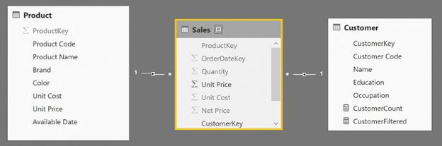
Figure A-8 Both relationships are set to their default mode, which is unidirectional.
The CROSSFILTER function enables bidirectional filtering for the duration of the CALCULATE statement. During the evaluation of COUNTROWS ( Customer ), the filter will move from Sales to Customer to show only the customers who are referenced in Sales.
This technique is very convenient when you need, for example, to compute the number of customers who bought a product. In fact, the filter moves naturally from Product to Sales. Then, however, you need to use bidirectional filtering to let it flow to Customer by passing through Sales. For example, Figure A-9 shows two calculations. One has bidirectional filtering activated and the other uses the default filter propagation.