

Chapter 7. Analyzing date and time intervals
Chapter 4, “Working with date and time,” discussed time intelligence and calculations over time. This chapter will show you several models that, again, use time as the primary analytical tool. This time, however, we are not interested in discussing calculations like year-to-date (YTD) and year-over-year. Instead, we want to discuss scenarios in which time is the focus of the analysis, but not necessarily the main dimension used to slice. Thus, we will show you scenarios like computing the number of working hours in a period, the number of employees available in different time frames for various projects, and the number of orders currently being processed.
What makes these models different from a standard model? In a standard model, a fact is an atomic event that happened at a very precise point in time. In these models, on the other hand, facts are typically events with durations, and they extend their effect for some time. Thus, what you store in the fact table is not the date of the event, but the point in time when the event started. Then, you must work with DAX and with the model to account for the duration of the event.
Concepts like time, duration, and periods are present in these models. However, as you will see, the focus is not only on slicing by time, but also on analyzing the facts with durations. Having time as one of the numbers to aggregate or to consider during the analysis makes these models somewhat complex. Careful modeling is required.
Introduction to temporal data
Having read this book so far, you are very familiar with the idea of using a date dimension to slice your data. This allows you to analyze the behavior of facts over time, by using the date dimension to slice and dice your values. When we speak about facts, we usually think about events with numbers associated with them, such as the number of items sold, their price, or the age of a customer. But sometimes, the fact does not happen at a given point in time. Instead, it starts at a given point in time, and then its effect has a duration.
Think, for example, about a normal worker. You can model the fact that, on a given date, that worker was working, produced some amount of work, and earned a specific amount of money. All this information is stored as normal facts. At the same time, you might store in the model the number of hours that person worked, to be able to summarize them at the end of the month. In such a case, a simple
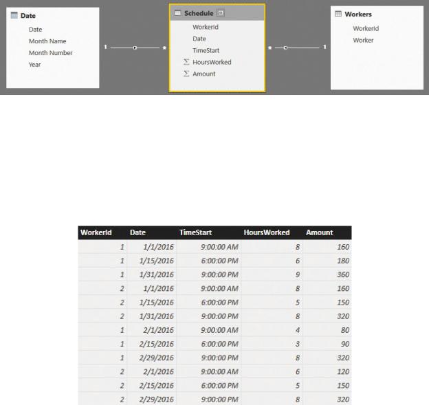
model like the one shown in Figure 7-1 looks correct. There, you have two dimensions, Workers and Date, and a Schedule fact table with the relevant keys and values.
FIGURE 7-1 This figure shows a simple data model for handling working schedules.
It might be the case that workers are paid at a different rate, depending on the time of the day. Night shifts, for example, are typically paid more than day shifts. You can see this effect in Figure 7-2, which shows the Schedule table content, where the hourly wage for shifts starting after 6:00 p.m. is higher. (You can obtain such a rate dividing Amount by HoursWorked.)
FIGURE 7-2 This figure shows the contents of the Schedule table.
You can now use this simple dataset to build a report that shows the hours worked on a monthly basis and the amount earned by the workers. The matrix is shown in Figure 7-3.

FIGURE 7-3 This figure shows a simple matrix report on top of the schedule data model.
At first sight, the numbers look correct. However, look again at Figure 7-2, focusing your attention on the days at the end of each period (either January or February). You’ll notice that at the end of January, the shifts start at 9:00 p.m., and because of their duration, they extend into the next day. Moreover, because it is the end of the month, they also extend to the next month. It would be much more accurate to state that some of the amount of January 31st needs to be accounted for in February, and some of the amount of February 29th needs to be accounted for in March. The data model does not produce this result. Instead it looks like all the hours are being worked in the day that the shift started, even if we know this is not the case.
Because this is only an introductory section, we do not want to dive into the details of the solution. These will be shown throughout the rest of the chapter. The point here is that the data model is not accurate. The problem is that each of the events stored in the fact table has a duration, and this duration extends its effects outside of the granularity that is defined in the fact table itself. In other words, the fact table has a granularity at the day level, but the facts it stores might contain information related to different days. Because of this, we have (again!) a granularity issue. A very similar scenario happens whenever you have to analyze durations. Each fact that has a duration falls into a similar scenario and needs to be handled with a lot of care. Otherwise, you end up with a data model that does not accurately represent the real world.
This is not to say that the data model is wrong. It all depends on the kinds of questions you want your data model to answer. The current model is totally fine for many reports, but it is not accurate enough for certain kinds of analysis. You might decide that the full amount should be shown in the month when the shift starts, and in most scenarios, this would be perfectly reasonable. However, this is a book about data modeling, so we need to build the right model for different requirements.
In this chapter, we will deal with scenarios like the one in the example, carefully studying how to model them to correctly reflect the data they need to
store.
Aggregating with simple intervals
Before diving into the complexity of interval analysis, let us start with some simpler scenarios. In this section, we want to show you how to correctly define a time dimension in your model. In fact, most of the scenarios we are managing require time dimensions, and learning how to model them is very important.
In a typical database, you will find a DateTime column that stores both the date and the time in the same column. Thus, an event that started at 09:30 a.m. on January 15, 2017 will contain a single column with that precise point in time. Even if this is the data you find in the source database, we urge you to split it into two different columns in your data model: one for the date and one for the time. The reason is that Tabular, which is the engine of both Power Pivot and Power BI, works much better with small dimensions than with larger ones. If you store date and time in the same column, you will need a much larger dimension because, for every single day, you need to store all the different hours and minutes. By splitting the information into two columns, the date dimension contains only the day granularity, and the time dimension contains only the time granularity. To host 10 years of data, for example, you need around 3,650 rows in the date dimension, and 1,440 rows in the time dimension, if you are working at the individual minute level. On the other hand, a single date/time dimension would require around 5,256,000 rows, which is 3,650 times 1,440. The difference in terms of query speed is tremendous.
Of course, you need to perform the operation of splitting the date/time column into two columns before the data enters your model. In other words, you can load a date/time column in your model, and then build two calculated columns on which to base the relationship—one for the date and one for the time. With that said, the memory used for the date/time column is basically a waste of resources because you will never use that column. You can obtain the same result with much less memory consumption by performing the split using the Excel or Power BI Query Editor or, for more advanced users, using a SQL view that performs the splitting. Figure 7-4 shows a very simple time dimension.

FIGURE 7-4 This figure shows a very basic time dimension at the minute granularity.
If the time dimension contained only hours and minutes, it would not be of much use unless you needed to perform an analysis at a very detailed level. You are likely to add some attributes to the dimension to be able to group the data in different buckets. For example, in Figure 7-5, we added two columns so we could group the time in day periods (night, morning, and so on) and in hourly buckets. We then reformatted the Time column.
FIGURE 7-5 You can group time in different buckets by using simple calculated columns.
You must take particular care when analyzing time buckets. In fact, even if it looks very natural to define a time dimension at the minute level and then group it using buckets, you may be able to define the dimension at the bucket level. In other words, if you are not interested in analyzing data at the minute level (which will usually be the case), but only want to perform an analysis at the half-hour level,