

Reallocating factors and percentages
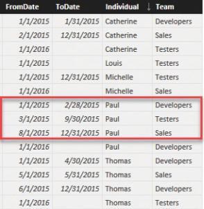
As the report in Figure 8-15 showed, it looks like Paul accounted for 62 hours in August for both the Sales and the Testers teams. These figures are clearly wrong. Paul cannot have worked for both teams at the same time. In this scenario—that is, when the many-to-many relationship generates overlaps—it is usually a good practice to store in the relationship a correction factor that indicates how much of Paul’s total time is to be allocated to each team. Let us see the data in more detail with the aid of Figure 8-16.
FIGURE 8-16 In August and September 2015, Paul is working for Testers and Sales.
The data in this model does not look correct. To avoid assigning 100 percent of Paul’s time to both teams, you can add a value to the bridge table that represents the percentage of time that needs to be assigned to each team. This requires splitting and storing the periods in multiple rows, as shown in Figure 8-17.
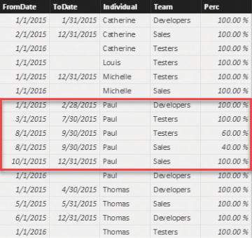
FIGURE 8-17 By duplicating some rows, you can avoid overlaps, and you can add percentages that allocate the hours.
Now Paul’s overlapping periods are divided into non-overlapping periods. In addition, a percentage was added to indicate that 60 percent of the total time should be allocated to the Testers team and 40 percent of the total time should be allocated to the Sales team.
The final step is to take these numbers into account. To do that, it is enough to modify the code of the measure so it uses the percentage in the formula. The final code is as follows:
Click here to view code image
HoursWorked := SUMX (
ADDCOLUMNS ( SUMMARIZE (
IndividualsTeams,
Individuals[IndividualKey],
IndividualsTeams[FromDate],
IndividualsTeams[ToDate],
IndividualsTeams[Perc]
),
"FirstDate", [FromDate],
"LastDate", IF ( ISBLANK ( [ToDate] ), MAX (
), CALCULATE (
SUM ( WorkingHours[Hours] ),
DATESBETWEEN ( 'Date'[Date], [FirstDate], [L VALUES ( 'Date'[Date] )
) * IndividualsTeams[Perc]
)
As you can see, we added the Perc column to SUMMARIZE. We then used it as a multiplier in the final step of the formula to correctly allocate the percentage of hours to the team. Needless to say, this operation made the code even harder than before.
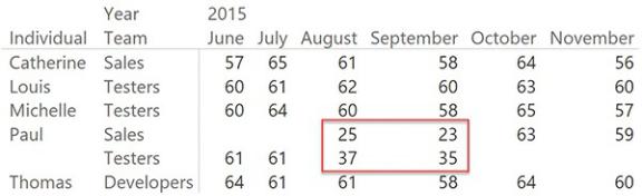
In Figure 8-18, you can see that in August and September, Paul’s hours are correctly split between the two teams he worked with.
FIGURE 8-18 The report shows correctly that Paul was in two teams in August and September, and splits hours between them.
Nevertheless, in doing this operation, we moved to a slightly different data model that transformed the overlapping periods into percentages. We had to do this because we did not want to obtain a non-additive measure. In fact, while it is true that many-to-many relationships are non-additive, it is also true that, in this specific case, we wanted to guarantee additivity because of the data we are representing.
From the conceptual point of view, this important step helps us introduce the next step in the optimization of the model: the materialization of many-to-many relationships.
Materializing many-to-many
As you saw in the previous examples, many-to-many relationships could have
temporal data (or, in general, with a complex filter), percentages, and allocation factors. That tends to generate very complex DAX code. In the DAX world, complex typically means slow. In fact, the previous expressions are fine if you need to handle a small volume of data, but for larger datasets or for heavy environments, they are too slow. The next section covers some performance considerations with many-to-many relationships. In this section, however, we want to show you how you can get rid of many-to-many relationships if you are seeking better performance, and as usual, easier DAX.
As we anticipated, most of the time, you can remove many-to-many relationships from the model by using the fact table to store the relationship between the two dimensions. In fact, in our example, we have two different dimensions: Teams and Individuals. They are linked by a bridge table, which we need to traverse and filter every time we want to slice by team. A more efficient solution would be to store the team key straight in the fact table by materializing the many-to-many relationship in the fact table.
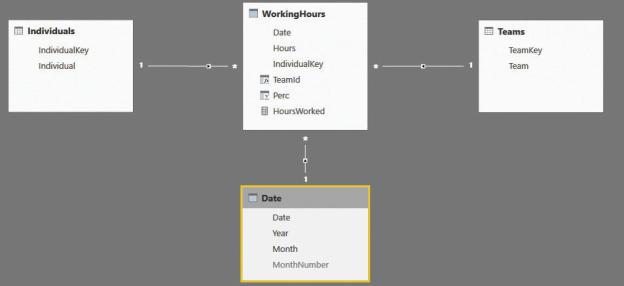
Materializing the many-to-many relationship requires that you denormalize the columns from the bridge table to the fact table, and at the same time increase the number of rows in the fact table. In the case of Paul’s hours that need to be assigned to two different teams during August and September, you will need to duplicate the rows, adding one row for each team. The final model will be a perfect star schema, as shown in Figure 8-19.
FIGURE 8-19 Once you remove the many-to-many relationship, you obtain a normal star schema.
Increasing the row count requires some steps of ETL. This is usually done