reasonable level of denormalization no matter how the original data is stored. As you’ve seen, if you denormalize too much, you face the problem of granularity. Later in this book, you will see that over-denormalizing a model has other negative consequences, too. What is, then, the correct level of denormalization?

There is no defined rule on how to obtain the perfect level of denormalization. Nevertheless, intuitively, you denormalize up to the point where a table is a selfcontained structure that completely describes the entity it stores. Using the example discussed in this section, you should move the Product Category and Product Subcategory columns in the Product table because they are attributes of a product, and you do not want them to reside in separate tables. But you do not denormalize the product in the Sales table because products and sales are two different pieces of information. A sale is pertinent to a product, but there is no way a sale can be completely identified with a product.

At this point, you might think of the model with a single table as being overdenormalized. That is perfectly true. In fact, we had to worry about product attribute granularity in the Sales table, which is wrong. If the model is designed the right way, with the right level of denormalization, then granularity comes out in a very natural way. On the other hand, if the model is over-denormalized, then you must worry about granularity, and you start facing issues.

Introducing star schemas

So far, we have looked at very simple data models that contained products and sales. In the real world, few models are so simple. In a typical company like Contoso, there are several informational assets: products, stores, employees, customers, and time. These assets interact with each other, and they generate events. For example, a product is sold by an employee, who is working in a store, to a particular customer, and on a given date.

Obviously, different businesses manage different assets, and their interactions generate different events. However, if you think in a generic way, there is almost always a clear separation between assets and events. This structure repeats itself in any business, even if the assets are very different. For example, in a medical environment, assets might include patients, diseases, and medications, whereas an event is a patient being diagnosed with a specific disease and obtaining a medication to resolve it. In a claim system, assets might include customers, claims, and time, while events might be the different statuses of a claim in the process of being resolved. Take some time to think about your specific business. Most likely, you will be able to clearly separate between your assets and events.

This separation between assets and events leads to a data-modeling technique known as a star schema. In a star schema, you divide your entities (tables) into two categories:

Dimensions A dimension is an informational asset, like a product, a customer, an employee, or a patient. Dimensions have attributes. For example, a product has attributes like its color, its category and subcategory, its manufacturer, and its cost. A patient has attributes such as a name, address, and date of birth.

Facts A fact is an event involving some dimensions. In Contoso, a fact is the sale of a product. A sale involves a product, a customer, a date, and other dimensions. Facts have metrics, which are numbers that you can aggregate to obtain insights from your business. A metric can be the quantity sold, the sales amount, the discount rate, and so on.

Once you mentally divide your tables into these two categories, it becomes clear that facts are related to dimensions. For one individual product, there are many sales. In other words, there is a relationship involving the Sales and Product tables, where Sales is on the many side and Product is on the one side. If you design this schema, putting all dimensions around a single fact table, you obtain the typical figure of a star schema, as shown in Figure 1-12 in Power Pivot’s diagram view.

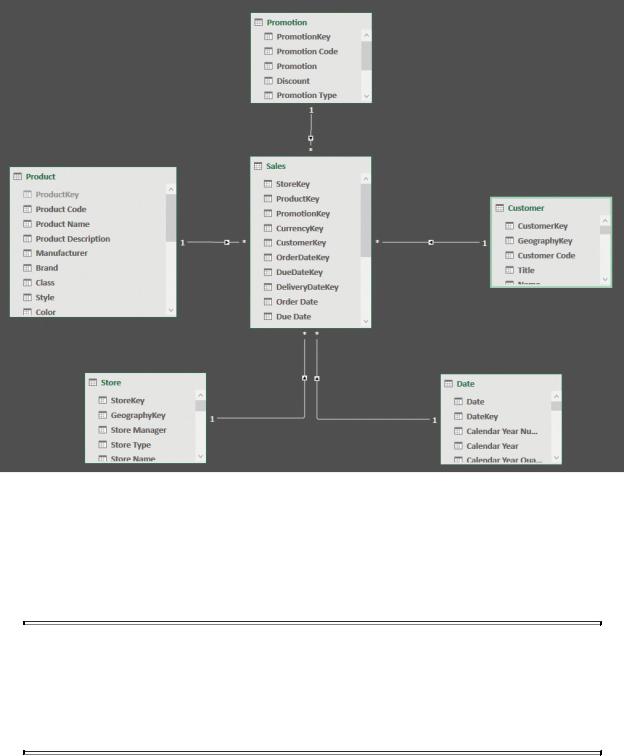
FIGURE 1-12 A star schema becomes visible when you put the fact table in the center and all the dimensions around it.

Star schemas are easy to read, understand, and use. You use dimensions to slice and dice the data, whereas you use fact tables to aggregate numbers. Moreover, they produce a small number of entries in the PivotTable field list.

Note

Star schemas have become very popular in the data warehouse industry. Today, they are considered the standard way of representing analytical models.

Because of their nature, dimensions tend to be small tables, with fewer than 1,000,000 rows—generally in the order of magnitude of a few hundred or thousand. Fact tables, on the other hand, are much larger. They are expected to store tens—if not hundreds of millions—of rows. Apart from this, the structure of

star schemas is so popular that most database systems have specific optimizations that are more effective when working with star schemas.

Tip

Before reading further, spend some time trying to figure out how your own business model might be represented as a star schema. You don’t need to build the perfect star schema right now, but it is useful to try this exercise, as it is likely to help you focus on a better way to build fact tables and dimensions.

It is important to get used to star schemas. They provide a convenient way to represent your data. In addition, in the business intelligence (BI) world, terms related to star schemas are used very often, and this book is no exception. We frequently write about fact tables and dimensions to differentiate between large tables and smaller ones. For example, in the next chapter, we will cover the handling of header/detail tables, where the problem is more generically that of creating relationships between different fact tables. At that point, we will take for granted that you have a basic understanding of the difference between a fact table and a dimension.

Some important details about star schemas are worth mentioning. One is that fact tables are related to dimensions, but dimensions should not have relationships among them. To illustrate why this rule is important and what happens if you don’t follow it, suppose we add a new dimension, Geography, that contains details about geographical places, like the city, state, and country/region of a place. Both the Store and Customer dimensions can be related to Geography. You might think about building a model like the one in Figure 1-13, shown in Power Pivot’s diagram view.

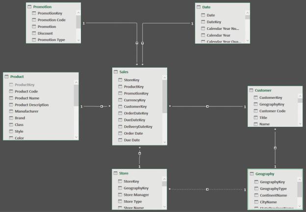
FIGURE 1-13 The new dimension, called Geography, is related to both the Customer and Store dimensions.

This model violates the rule that dimensions cannot have relationships between them. In fact, the three tables, Customer, Store, and Geography, are all dimensions, yet they are related. Why is this a bad model? Because it introduces ambiguity.

Imagine you slice by city, and you want to compute the amount sold. The system might follow the relationship between Geography and Customer, returning the amount sold, sliced by the city of the customer. Or, it might follow the relationship between Geography and Store, returning the amount sold in the city where the store is. As a third option, it might follow both relationships, returning the sales amount sold to customers of the given city in stores of the given city. The data model is ambiguous, and there is no easy way to understand what the number will be. Not only this is a technical problem, it is also a logical one. In fact, a user looking at the data model would be confused and unable to understand the numbers. Because of this ambiguity, neither Excel nor Power BI let you build such a model. In further chapters, we will discuss ambiguity to a greater extent. For now, it is important only to note that Excel (the tool we used to build this

example) deactivated the relationship between Store and Geography to make sure that the model is not ambiguous.

You, as a data modeler, must avoid ambiguity at all costs. How would you resolve ambiguity in this scenario? The answer is very simple. You must denormalize the relevant columns of the Geography table, both in Store and in Customer, removing the Geography table from the model. For example, you could include the ContinentName columns in both Store and in Customer to obtain the model shown in Figure 1-14 in Power Pivot’s diagram view.

FIGURE 1-14 When you denormalize the columns from Geography, the star schema shape returns.

With the correct denormalization, you remove the ambiguity. Now, any user will be able to slice by columns in Geography using the Customer or Store table. In this case, Geography is a dimension but, to be able to use a proper star schema, we had to denormalize it.

Before leaving this topic, it is useful to introduce another term that we will use often: snowflake. A snowflake is a variation of a star schema where a dimension is not linked directly to the fact table. Rather, it is linked through another dimension. You have already seen examples of a snowflake; one is in Figure 1-15, shown in Power Pivot’s diagram view.

FIGURE 1-15 Product Category, Subcategory, and Product form a chain of relationships and are snowflaked.

Do snowflakes violate the rule of dimensions being linked together? In some sense, they do, because the relationship between Product Subcategory and Product is a relationship between two dimensions. The difference between this example and the previous one is that this relationship is the only one between Product Subcategory and the other dimensions linked to the fact table or to Product. Thus, you can think of Product Subcategory as a dimension that groups different products together, but it does not group together any other dimension or fact. The same, obviously, is true for Product Category. Thus, even if snowflakes violate the aforementioned rule, they do not introduce any kind of ambiguity, and a data model with snowflakes is absolutely fine.

Note

You can avoid snowflakes by denormalizing the columns from the farthest tables into the one nearer to the fact table. However, sometimes snowflakes are a good way of representing your data and —apart from a small performance degradation—there is nothing wrong with them.

As you will see throughout this book, star schemas are nearly always the best way to represent your data. Yes, there are some scenarios in which star schemas are not the perfect way to go. Still, whenever you work with a data model, representing it with a star schema is the right thing to do. It might not be perfect, but it will be near-to-perfect enough to be a good solution.