

FIGURE 4-17 Delivered Amount uses the relationship based on a delivery date, but its logic is hidden in the measure.
Thus, the simple rule is to create a single date dimension for the whole model. Obviously, this is not a strict rule. There are scenarios where having multiple date dimensions makes perfect sense. But there must be a powerful need to justify the pain of handling multiple Date tables.
In our experience, most data models do not really require multiple Date tables. One is enough. If you need some calculations made using different dates, then you can create measures to compute them, leveraging inactive relationships. Most of the time, adding many date dimensions comes from some lack in the analysis of the requirements of the model. Thus, before adding another date dimension, always ask yourself whether you really need it, or if you can compute the same values using DAX code. If the latter is true, then go for more DAX code and fewer date dimensions. You will never regret that.
Handling date and time
Date is almost always a needed dimension in any model. Time, on the other hand, appears much less frequently. With that said, there are scenarios where both the date and the time are important dimensions, and in those cases, you need to carefully understand how to handle them.
The first important point to note is that a Date table cannot contain time information. In fact, to mark a table as a Date table (which you must do if you intend to use any time-intelligence functions on a table), you need to follow the requirements imposed by the DAX language. Among those requirements is that the column used to hold the datetime value should be at the day granularity, without time information. You will not get an error from the engine if you use a Date table that also contains time information. However, the engine will not be able to correctly compute time-intelligence functions if the same date appears multiple times.
So what can you do if you need to handle time too? The easiest and most efficient solution is to create one dimension for the date and a separate dimension for the time. You can easily create a time dimension by using a simple piece of M code in Power Query, like the following:
Click here to view code image
Let
StartTime = #datetime(1900,1,1,0,0,0),
Increment = #duration(0,0,1,0),
Times = List.DateTimes(StartTime, 24*60, Increme TimesAsTable = Table.FromList(Times,Splitter.Spl RenameTime = Table.RenameColumns(TimesAsTable,
{{"Column1", "Time"}}),
ChangedDataType = Table.TransformColumnTypes(Ren {{"Time", type time}}),
AddHour = Table.AddColumn( ChangedDataType, "Hour",
each Text.PadStart(Text.From(Time.Hour([Time
),
AddMinute = Table.AddColumn( AddHour,
"Minute",
each Text.PadStart(Text.From(Time.Minute([Ti
),
AddHourMinute = Table.AddColumn( AddMinute,
"HourMinute", each [Hour] & ":" & [Minute]
),
AddIndex = Table.AddColumn( AddHourMinute, "TimeIndex",
each Time.Hour([Time]) * 60 + Time.Minute([T
),
Result = AddIndex
in
Result
The script generates a table like the one shown in Figure 4-18. The table contains a TimeIndex column (with the numbers from 0 to 1439), which you can use to link the fact table, and a few columns to slice your data. If your table contains a different column for the time, you can easily modify the previous script to generate a time as the primary key.
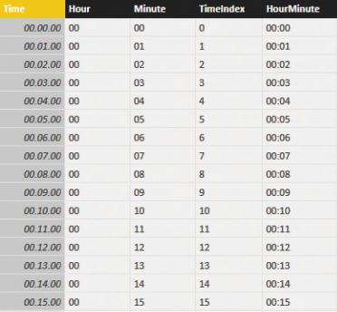
FIGURE 4-18 This is a simple time table that is generated with Power Query.
The time index is computed by multiplying the hours by 60 and adding the minutes, so it can be easily included as a key in your fact table. This calculation should be done in the data source that feeds the table.
Using a separate time table lets you slice data by hours, minutes, or different columns that you might add to the time table. Frequent options are periods of the day (morning, afternoon, or night) or time ranges—for example hourly ranges, like the ones we used in the report in Figure 4-19.

FIGURE 4-19 The time dimension is useful to generate reports that show sales divided by hour, for example.
There are scenarios, however, where you do not need to stratify numbers by time ranges. For example, you might want to compute values based on the difference in hours between two events. Another scenario is if you need to compute the number of events that happened between two timestamps, with a granularity below the day. For example, you might want to know how many customers entered your shop between 8:00 a.m. on January 1st and 1:00 p.m. on January 7th. These scenarios are a bit more advanced, and they are covered in Chapter 7, “Analyzing date and time intervals.”
Time-intelligence calculations
If your data model is prepared in the correct way, time-intelligence calculations are easy to author. To compute time intelligence, you need to apply a filter on the Calendar table that shows the rows for the period of interest. There is a rich set of functions that you can use to obtain these filters. For example, a simple YTD can be written as follows:
Click here to view code image
Sales YTD :=
CALCULATE (
[Sales Amount],
DATESYTD ( 'Date'[Date] )
)
DATESYTD returns the set of dates starting from the 1st of January of the currently selected period and reaching the last date included in the context. Other useful functions are SAMEPERIODLASTYEAR, PARALLELPERIOD, and
LASTDAY. You can combine these functions to obtain more complex aggregations.
For example, if you need to compute YTD of the previous year, you can use the following formula:
Click here to view code image
Sales PYTD := CALCULATE (
[Sales Amount],
DATESYTD ( SAMEPERIODLASTYEAR ( 'Date'[Date] ) )
)
Another very useful time-intelligence function is DATESINPERIOD, which returns the set of dates in a given period. It can be useful for computing moving averages, like in the following example, where DATESINPERIOD returns the last 12 months, using the last date in the filter context as a reference point:
Click here to view code image
Sales Avg12M := CALCULATE (
[Sales Amount] / COUNTROWS ( VALUES ( 'Date'[Mon DATESINPERIOD (
'Date'[Date],
MAX ( 'Date'[Date] ), -12,
MONTH
)
)
You can see the result of this average in Figure 4-20.