

like the total amount sold can still be recovered from the original fact table. Thus, we are not losing expressivity in the model. Instead, we are increasing it by adding fact tables when needed. Figure 7-24 shows you the whole model we built in this section. Obviously, you will never build all these tables in a single model. The intent is only to show all the fact tables we created in this long journey to analyze how open orders can co-exist and provide different insights in your model.
FIGURE 7-24 The whole model, with all the fact tables together, is pretty complex.
Depending on the size of your data model and the kind of insights you need, you will build only parts of this whole model. As we have said multiple times, the intent is to show you different ways to build a data model and how the DAX code becomes easier or harder depending on how well the model fits your specific needs. Along with the DAX code, flexibility also changes in each approach. As a data modeler, it is your task to find the best balance and, as always, to be prepared to change the model if the analytical needs change.
Mixing different durations
When handling time and duration, you will sometimes have several tables that contain information that is valid for some period in time. For example, when handling employees, you might have two tables. The first table contains the store
at which the employee is working and an indication of when this is happening. The second one might come from a different source and contain the gross salary of the employee. The start and end date of the two tables do not need to match. The employee’s salary could change on one date, and the employee could switch to a different store on a different date.
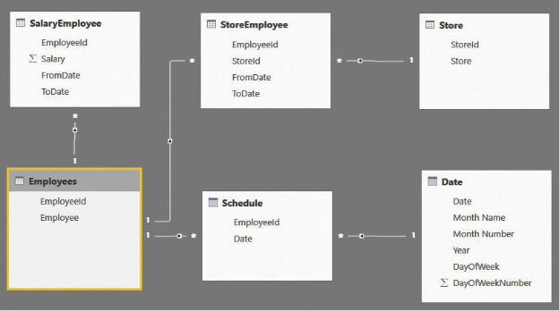
If you face such a scenario, then you can either write very complex DAX code to solve it or change the data model so it stores the correct information and makes the code much easier to use. Let us start by looking at the data model shown in Figure 7-25.
FIGURE 7-25 This data model shows employees with different store assignments and different salaries.
This time, the model is somewhat complex. A more complete description follows:
 SalaryEmployee This contains the salary of an employee, with the start and end date. Thus, each salary has a duration.
 StoreEmployee This contains the store assignment of an employee, again with the start and end date. Thus, there is also a duration in this case, which might be different from the one in SalaryEmployee.
 Schedule This contains the days that the employee worked.
The other tables (Store, Employees, and Date) are simple tables containing
employee names, store names, and a standard calendar table.
The data model contains all the necessary information to produce a report that shows, over time, the amount paid to the employee. It gives the user the ability to slice by store or by employee. With that said, the DAX measures that you must write are very complex because, given a date, you must perform the following:
1.Retrieve the salary that was effective on the date by analyzing FromDate and ToDate in SalaryEmployee of the given employee. If the selection contains multiple employees, then you will need to perform this operation for each employee separately, one by one.
2.Retrieve the store that was assigned to the employee at the given time.
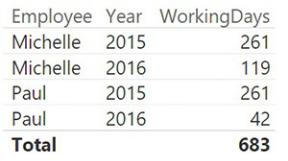
Let us start with a simple report that works straight out of the model: the number of working days per employee, sliced by year. It works because the relationships are set so you can slice Schedule based on both the calendar year and the employee name. You can author a simple measure like the following:
Click here to view code image
WorkingDays := COUNTROWS ( Schedule )
With the measure in place, the first part of the report is straightforward, as shown in Figure 7-26.
FIGURE 7-26 This figure shows the number of working days, sliced by year and employee.
First, let us determine the amount paid to Michelle, who is employee 2, in 2015. The SalaryEmployee table with the salaries contains the values shown in Figure 7-27.
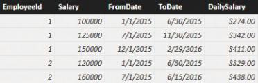
FIGURE 7-27 Depending on the date, the salary changes for each employee.
Michelle has two different salary amounts in 2015. Thus, the formula needs to iterate on a day-by-day basis and determine what the current daily salary was for each day. This time, you cannot rely on relationships because the relationships must be based on a between condition. The salary has a range defined by FromDate and ToDate columns, including the current date.
The code is not exactly easy to write, as you can see in the following measure definition:
Click here to view code image
SalaryPaid = SUMX (
'Schedule',
VAR SalaryRows =
FILTER ( SalaryEmployee, AND (
SalaryEmployee[EmployeeId] = Schedul AND (
SalaryEmployee[FromDate] <= Sche SalaryEmployee[ToDate] > Schedul
)
)
)
RETURN
IF ( COUNTROWS ( SalaryRows ) = 1, MAXX ( Sa
)
The complexity comes from the fact that you must move the filter through a complex FILTER function that evaluates the between condition. Additionally, you must make sure that a salary exists and is unique, and you must verify your findings before returning them as the result of the formula. The formula works,
provided the data model is correct. If, for any reason, the dates of the salary table overlap, then the result might be wrong. You would need further logic to check it and to correct the possible error.
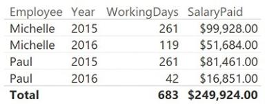
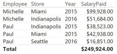
With this code in place, you can enhance the report, displaying the salary paid in each period, as shown in Figure 7-28.
FIGURE 7-28 This figure shows the number of working days, sliced by year and employee.
The scenario becomes more complex if you want to be able to slice by store. In fact, when you slice by store, you want to account for only the period when each employee was working for the given store. You must consider the filter on the store and use it to filter only the rows from Schedule when the employee was working there. Thus, you must add a FILTER around the Schedule table by using the following code:
Click here to view code image
SalaryPaid = SUMX (
FILTER ( 'Schedule', AND (
Schedule[Date] >= MIN ( StoreEmployee[Fr Schedule[Date] <= MAX ( StoreEmployee[To
)
),
VAR SalaryRows =
FILTER ( SalaryEmployee, AND (
SalaryEmployee[EmployeeId] = Schedul AND (
SalaryEmployee[FromDate] <= Sche SalaryEmployee[ToDate] > Schedul
)
)
)
RETURN
IF ( COUNTROWS ( SalaryRows ) = 1, MAXX ( Sa
)
This formula works correctly, as shown in Figure 7-29, but it is extremely complex and might return incorrect results if it is not used in the proper way.
FIGURE 7-29 The last version of SalaryPaid returns the correct numbers when sliced by store.
The problem with this model is that the relationship between stores, salary, and employees is complex. And using DAX to navigate through it results in very complex code, which is extremely error-prone. As before, the solution is to move complexity from the DAX code to the loading process, moving toward a star schema.
For each row in Schedule, you can easily compute which store the employee is working at and what the daily salary for that day of work is. As always, a correct denormalization removes complexity from the aggregation formulas, moving it to the fact table and resulting in a much simpler model to work with.
You should create two calculated columns in Schedule: one containing the daily salary and another containing the store ID. You can do this by using the following code:
Click here to view code image
Schedule[DailySalary] =
VAR CurrentEmployeeId = Schedule[EmployeeId]
VAR CurrentDate = Schedule[Date] RETURN
CALCULATE (
VALUES ( SalaryEmployee[DailySalary] ), SalaryEmployee[EmployeeId] = CurrentEmployee SalaryEmployee[FromDate] <= CurrentDate, SalaryEmployee[ToDate] > CurrentDate
)
Schedule[StoreId] =
VAR CurrentEmployeeId = Schedule[EmployeeId] VAR CurrentDate = Schedule[Date]
RETURN CALCULATE (
VALUES ( StoreEmployee[StoreId] ), StoreEmployee[EmployeeId] = CurrentEmployeeI StoreEmployee[FromDate] <= CurrentDate, StoreEmployee[ToDate] >= CurrentDate
)
When the two columns are ready, you can get rid of most of the relationships with the SalaryEmployee and StoreEmployee tables, and you can transform the data model into the simpler star schema shown in Figure 7-30.
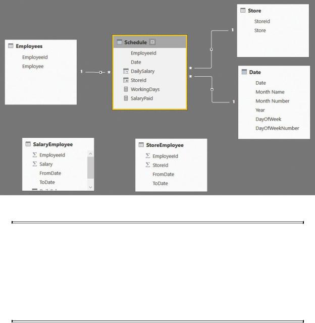
FIGURE 7-30 The denormalized model is a star schema.
 Note
Note
We intentionally left SalaryEmployee and StoreEmployee visible in the figure of the model to highlight the fact that these tables, which were used to compute the calculated columns, have no relationships with the remaining ones. In a production model, you would likely hide these tables to prevent users from even seeing them. They do not contain useful information from a user point of view.
With the new model, the code to compute the salary paid is as easy as the following one:
Click here to view code image
SalaryPaid = SUM ( Schedule[DailySalary] )
Once again, you have seen that a proper denormalization strategy leads to the best data model. Maintaining complex relationships in the model does not help the code, which tends to be very complex and error-prone. On the other hand, denormalizing the values by using SQL or DAX and calculated columns splits the