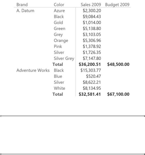
is not browsing below the granularity of Budget. The result is shown in Figure 9- 13, where Budget is correctly reported at the brand level, and is blanked at the color level.

FIGURE 9-13 This report blanks the value of Budget below the correct granularity.

Note

Whenever you have fact tables at different granularity, it is very important to recognize when a value should not be shown because of granularity issues. Otherwise, the report will always produce a number—and it is likely to be the wrong one.

Allocating values at a higher granularity

In the previous examples, you learned how to hide values when the user is browsing at a granularity that is no longer supported by the data model. This technique is useful to avoid showing a wrong number. For some specific scenarios, however, you can do more than this. You can compute the value at the higher granularity using an allocation factor. For example, suppose you do not

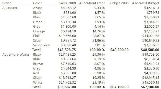
know the budget of blue products at a company called Adventure Works. (You only know the budget for the total of Adventure Works.) You can ascertain this by taking a percentage of the total budget, which you can compute on the fly. This percentage is the allocation factor.

A good allocation factor can be, for example, the percentage of sales of blue products against the totality of colors in the previous year. Rather than trying to describe it with words, it is much simpler to look at the final report shown in Figure 9-14.

FIGURE 9-14 The Allocated Budget column shows values at a higher granularity by computing them dynamically.

Let us examine Figure 9-14 in more detail. In previous figures, we used Sales 2009, whereas here we are showing Sales 2008. This is because we use Sales 2008 to compute the allocation factor, which is defined here as the amount of sales in 2008 of blue products divided by the amount of sales in 2008 at the Budget granularity.

You can see, for example, that blue products from Adventure Works made $8,603.64 in sales, which, divided by $93,587.00, results in 9.19% as the share of sales in 2008. The budget of blue products is not available in 2009, but you can compute it by multiplying the budget of Adventure Works products by the share in 2008, for an expected value of $6,168.64.

Computing the value is simple when you understand the granularity details. It is