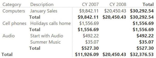
)

)

)

Using this formula, you can build reports like the one shown in Figure 4-38.

FIGURE 4-38 When using overlapping periods, you can browse different periods in the same year.

The report in Figure 4-38 shows the sales of different categories over different years, even if the periods overlap. In this case, the model remained fairly simple because we could not rely on changes in the model to make the code easier to write. You will see several examples similar to this one in Chapter 7, but in that chapter we will also create different data models to show how to write simpler (and maybe faster) code. In general, many-to-many relationships are powerful and easy to use, but writing the code to make them work is sometimes (like in this case) difficult.

The reason we wanted to show you this example is not to scare you or to show you a scenario where the model fails in making the code simple to write. It is simply that if you want to produce complex reports, sooner or later, you will need to author complex DAX code.

Working with weekly calendars

As you learned, as long as you work with standard calendars, you can easily compute measures like year-to-date (YTD), month-to-date (MTD), and the same period last year, because DAX offers you a set of predefined functions that perform exactly these types of calculation. This becomes much more complex as soon as you need to work with non-standard calendars, however.

What is a non-standard calendar? It is any kind of calendar that does not follow the canonical division of 12 months, with different days per month. For example, many businesses need to work with weeks instead of months. Unfortunately, weeks do not aggregate in months or years. In fact, a month is made of a variable number of weeks, as is a year. Moreover, there are some common techniques in the handling of weekly based years, but none are a standard that can be formalized in a DAX function. For this reason, DAX does not offer any functionality to handle non-standard calendars. If you need to manage them, you are on your own.

Luckily, even with no predefined function, you can leverage certain modeling techniques to perform time intelligence over non-standard calendars. This section does not cover them all. Our goal here is simply to show you some examples that you will probably need to adapt to your specific needs in the event you want to adopt them. If you are interested in more information about this topic, you will find a more complete treatment here: http://www.daxpatterns.com/time-patterns/.

As an example of non-standard calendar, you will learn how to handle weekly based calculations using the ISO 8601 standard. If you are interested in more information about this way of handling weeks, you can find it here: https://en.wikipedia.org/wiki/ISO_week_date.

The first step is to build a proper ISO Calendar table. There are many ways to build one. Chances are you already have a well-defined ISO calendar in your database. For this example, we will build an ISO calendar using standard DAX and a lookup table, as this provides a good opportunity to learn more modeling tricks.

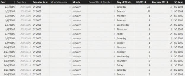
The calendar we are using is based on weeks. A week always starts on Monday, and a year always starts when its first week starts. Because of this, it is very likely that a year might start, for example, on the 29th of December of the previous year or on the 2nd of January of the current calendar year. To handle this, you can add calculated columns to a standard Calendar table to compute the ISO Week number and the ISO Year number. By using the following definitions, you will be able to create a table that contains Calendar Week, ISO Week, and ISO Year columns, as outlined in Figure 4-39:

Click here to view code image

'Date'[Calendar Week] = WEEKNUM ( 'Date'[Date], 2 ) 'Date'[ISO Week] = WEEKNUM ('Date'[Date], 21 ) 'Date'[ISO Year] =

CONCATENATE ( "ISO ", IF (

AND ( 'Date'[ISO Week] < 5, 'Date'[Calendar YEAR ( 'Date'[Date] ) + 1,

IF (

AND ( 'Date'[ISO Week] > 50, 'Date'[Cale YEAR ( 'Date'[Date] ) - 1,

YEAR ( 'Date'[Date] )

)

)

)

FIGURE 4-39 The ISO year is different from the calendar year because ISO years always start on Monday.

While the week and month can be easily computed with a simple calculated column, the ISO month requires a bit more attention. With the ISO standard, there are different ways to compute the month number. One is to start by dividing the four quarters. Each quarter has three months, and the months are built using one of three groupings: 445, 454, or 544. The digits in these numbers stand for the number of weeks to include in each month. For example, in 445, the first two months in a quarter contain four weeks, whereas the last month contains five weeks. The same concept applies to the other techniques. Instead of searching for a complex mathematical formula that computes the month to which a week belongs in the different standard, it is easier to build a simple lookup table like the one shown in Figure 4-40.

)

)

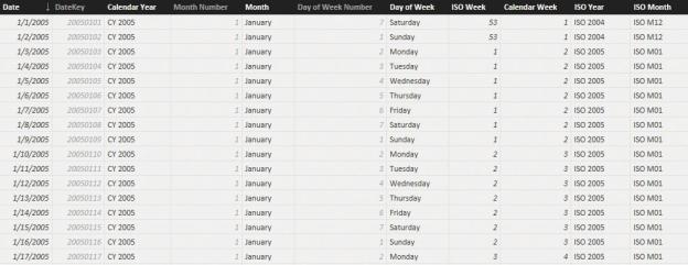
The resulting table contains the year and the month, as shown in Figure 4-41.

FIGURE 4-41 The ISO month is easily computed using a lookup table.

Now that all the columns are in place, you can easily build a hierarchy and start browsing your model splitting by ISO years, months, and weeks. Nevertheless, on such a calendar, computing values like YTD, MTD, and other time-intelligence calculations will prove to be a bit more challenging. In fact, the canonical DAX functions are designed to work only on standard Gregorian calendars. They are useless if your calendar is non-standard.

This requires you to build the time-intelligence calculations in a different way —that is, without leveraging the predefined functions. For example, to compute ISO YTD, you can use the following measure:

Click here to view code image

Sales ISO YTD := IF (

HASONEVALUE ( 'Date'[ISO Year] ), CALCULATE (

[Sales Amount],

ALL ('Date' ),

FILTER ( ALL ( 'Date'[Date] ), 'Date'[Date] VALUES ( 'Date'[ISO Year] )

)

)

As you can see, the core of the measure is the set of filters you need to apply to the Calendar table to find the correct set of dates that compose the YTD. Figure 4- 42 shows the result.

FIGURE 4-42 The ISO YTD measure computes YTD for the ISO calendar, which is a non-standard calendar.

Computing month-to-date (MTD), quarter-to-date (QTD), and measures using a similar pattern is indeed very easy. Things get a bit more complex, however, if you want to compute, for example, calculations like the same period last year. In fact, because you cannot rely on the SAMEPERIODLASTYEAR function, you need to work a bit more on both the data model and the DAX code.

To compute the same period last year, you need to identify the date currently selected in the filter context and then find the same set of dates in the previous year. You cannot use the Date column for this because the ISO date has a completely different structure than the calendar date. Thus, the first step is to add a new column to the Calendar table that contains the ISO day number in the year. This can be accomplished easily with the following calculated column:

Click here to view code image

Date[ISO Day Number] = ( 'Date'[ISO Week] - 1 ) * 7 + WEEKDAY( 'Date'[Date], 2 )

You can see the resulting column in Figure 4-43.

FIGURE 4-43 The ISO Day Number column shows the incremental number of days in the year, according to the ISO standard.

This column is useful because to find the same selected period in the last year, you can now use the following code:

Click here to view code image

Sales SPLY := IF (

HASONEVALUE ( 'Date'[ISO Year Number] ), CALCULATE (

[Sales Amount],

ALL ( 'Date' ),

VALUES ( 'Date'[ISO Day Number] ),

'Date'[ISO Year Number] = VALUES ( 'Date'[IS

1

)

)

As you can see, the formula removes all filters from the Date table and replaces them with two new conditions:

The ISO Year Number should be the current year reduced by one.

The ISO Day Numbers need to be the same.

In this way, no matter what selection you have made in the current filter context, it will be moved back by one year, regardless of whether it is a day, a week, or a month.

In Figure 4-44, you can see the Sales SPLY measure working with a report sliced by year and month.