Chapter 10. Segmentation data models

In Chapter 9, “Working with different granularity,” you learned how to model your data with standard relationships: two tables related based on a single column. At the end, many-to-many relationships were built using standard relationships. In this chapter, you will learn how to handle more complex relationships between tables by leveraging the DAX language. Tabular models can handle simple or bidirectional relationships between tables, which might look somewhat limited. However, by taking advantage of the DAX language, you can create very advanced models with basically any kind of relationship, including virtual ones. When it comes to solving complex scenarios, DAX plays an important role in the definition of the data model.

To demonstrate these kinds of relationships, we will use as examples some data models where the main topic is that of segmenting the data. Segmentation is a common modeling pattern that happens whenever you want to stratify your data based on some configuration table. Imagine, for example, that you want to cluster your customers based on the age range, your products based on the amount sold, or your customers based on the revenues generated.

The goal of this chapter is not to give you pre-built patterns that you can use in your model. Instead, we want to show you unusual ways of using DAX to build complex models, to broaden your understanding of relationships, and to let you experience what you can achieve with DAX formulas.

Computing multiple-column relationships

The first set of relationships we will show is calculated physical relationships. The only difference between this and a standard relationship is that the key of the relationship is a calculated column. In scenarios where the relationship cannot be set because a key is missing, or you need to compute it with complex formulas, you can leverage calculated columns to set up the relationship. Even if based on calculated columns, this will still be a physical relationship.

The Tabular engine only allows you to create relationships based on a single column. It does not support relationships based on more than one column. Yet, relationships based on multiple columns are very useful, and appear in many data models. If you need to work with these kinds of models, use the two following methods to do so:

Define a calculated column that contains the composition of the keys and use

it as the new key for the relationship.

Denormalize the columns of the target table (the one side in a one-to-many relationship) using the LOOKUPVALUE function.

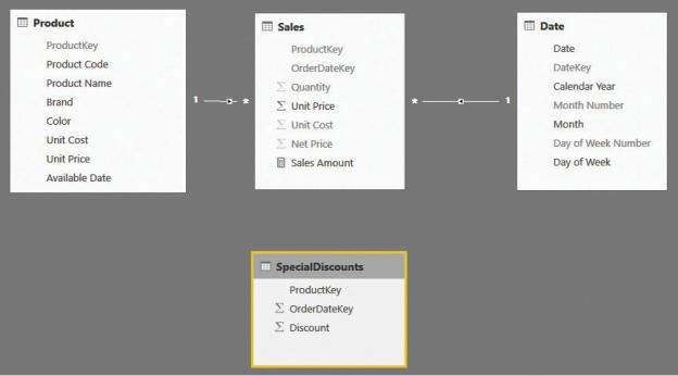
As an example, imagine you have a special “Product of the Day” promotion, where on some days, you make a special promotion for a single product with a given discount, as shown in Figure 10-1.

FIGURE 10-1 The SpecialDiscounts table needs a relationship based on two columns with Sales.

The table with the promotion (SpecialDiscounts) contains three columns: ProductKey, OrderDateKey, and Discount. If you need to use this information to compute, for example, the amount of the discount, you face the problem that for any given sale, the discount depends on ProductKey and OrderDateKey. Thus, you cannot create the relationship between Sales and SpecialDiscounts, because it would involve two columns, and Tabular supports only single-column relationships.

To find a possible solution to this scenario, consider that nothing prevents you from creating a relationship based on a calculated column. In fact, if the engine does not support a relationship based on two columns, you can build a new column that contains both, and then build a relationship on top of this new column. You can create a new calculated column in both the SpecialDiscount and Sales tables that contains the combination of the two columns by using the following

code:

Click here to view code image

Sales[SpecialDiscountKey] = Sales[ProductKey] & "-"

& Sales[OrderDateKey]

You use a similar expression in SpecialDiscount. After you define the two columns, you can finally create the relationship between the two tables. This results in the model shown in Figure 10-2.

FIGURE 10-2 You can use the calculated column as the basis of the relationship.

This solution is straightforward and works just fine. However, there are several scenarios where this is not the best solution because it requires you to create two calculated columns that might have many different values. From a performance point of view, this is not advisable.

Another possible solution to the same scenario is to use the LOOKUPVALUE function. Using LOOKUPVALUE, you can denormalize the discount directly in the fact table by defining a new calculated column in Sales that contains the following

code:

Click here to view code image

Sales[SpecialDiscount] = LOOKUPVALUE (

SpecialDiscounts[Discount], SpecialDiscounts[ProductKey], Sales[ProductKey], SpecialDiscounts[OrderDateKey], Sales[OrderDateK

)

Following this second pattern, you do not create any relationship. Instead, you move the Discount value in the fact table, performing a lookup. In a more technical way, we say you denormalized the SpecialDiscount value from the SpecialDiscounts table into Sales.

Both options work fine, and the choice between them depends on several factors. If Discount is the only column you need to use from the SpecialDiscount table, then denormalization is the best option. Only a single calculated column is created, with fewer distinct values, comparatively to two calculated columns with many more distinct values. Thus, it reduces memory usage and makes the code simpler to author.

If, on the other hand, SpecialDiscounts contains many columns that you need to use in your code, then each of them would have to be denormalized in the fact table, resulting in a waste of memory and, possibly, in worse performance. In that case, the calculated column with the new composite key would be a superior method.

This first simple example is important because it demonstrates a common and important feature of DAX: the ability to create relationships based on calculated columns. This capability shows that you can create any kind of relationship, as long as you can compute it and materialize it in a calculated column. In the next example, we will show you how to create relationships based on static ranges. By extending the concept, you can create almost any kind of relationship.

Computing static segmentation

Static segmentation is a very common scenario where you have a value in a table, and, rather than being interested in the analysis of the value itself (as there might be hundreds or thousands of possible values), you want to analyze it by splitting the value into segments. Two very common examples are the analysis of sales by customer age or by list price. It is pointless to partition sales amounts by all

unique values of list price because there are too many different values in list price. However, if you group different prices in ranges, then it may be possible to obtain good insight from the analysis of these groups.

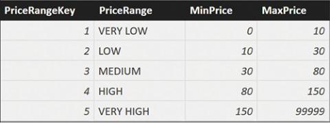
In this example, you have a table, PriceRanges, that contains the price ranges. For each range, you define the boundaries of the range itself, as shown in Figure 10-3.

FIGURE 10-3 This is the configuration table for the price ranges.

Here, as in the previous example, you cannot create a direct relationship between the fact table, containing sales, and the PriceRanges configuration table. This is because the key in the configuration table depends on a range relationship, and range relationships are not supported by DAX. In this case, the best solution is to denormalize the price range directly in the fact table by using a calculated column. The pattern of the code is similar to the previous one, with the main difference being the following formula:

Click here to view code image

Sales[PriceRange] = CALCULATE (

VALUES ( PriceRanges[PriceRange] ), FILTER (

PriceRanges, AND (

PriceRanges[MinPrice] <= Sales[Net Price PriceRanges[MaxPrice] > Sales[Net Price]

)

)

)

It is interesting to note the use of VALUES in this code to retrieve a single

value. VALUES returns a table, not a value. However, whenever a table contains a single row and a single column, it is automatically converted into a scalar value, if needed by the expression.

Because of the way FILTER computes its result, it will always return a single row from the configuration table. Thus, VALUES is guaranteed to always return a single row, and the result of CALCULATE is the description of the price range containing the current net price. Obviously, this expression works fine if the configuration table is well designed. However, if for any reason the ranges contain holes or overlap, then VALUES will return many rows, and the expression might result in an error.

A better way to author the previous code is to leverage the error-handling function, which will detect the presence of a wrong configuration, and return an appropriate message, as in the following code:

Click here to view code image

Sales[PriceRange] =

VAR ResultValue =

CALCULATE ( IFERROR (

VALUES ( PriceRanges[PriceRange] ), "Overlapping Configuration"

), FILTER (

PriceRanges, AND (

PriceRanges[MinPrice] <= Sales[Net P PriceRanges[MaxPrice] > Sales[Net Pr

)

)

)

RETURN IF (

ISEMPTY ( ResultValue ),

"Wrong Configuration", ResultValue

)

This code detects both overlapping values (with the internal IFERROR) and holes in the configuration (by checking the result value with ISEMPTY before