

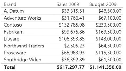
FIGURE 9-6 Because the model is based on a star schema, it now produces meaningful numbers.
The problem with this solution is that to make it work, we had to pay a huge price in terms of analytical power. That is, we had to remove all the detailed information about sales. On the date, for example, we had to restrict data to only 2009. In addition, we are no longer able to slice the sales by month and quarter, or by product color. Thus, even if the solution works from a technical point of view, it is far from being correct. What we would like to achieve is a way to slice the budget without losing any analytical capability in Sales.
Using DAX code to move filters
The next technique we want to analyze to solve the scenario is based on DAX. The problem with the data model in Figure 9-3 is that you can filter by brand using the Brand column in the Product table, but because there are no relationships between Product and Budget, the filter will not be able to reach the Budget table.
By using a DAX filter, you can force the filter from the Brand column in Products to the Brand column in Budget. The filter must be written in different ways, depending on the version of DAX you have available. In Power BI and Excel 2016 and later, you can leverage set functions. In fact, if you author the code of the Budget 2009 measure by using the following expression, it will correctly slice by brand and country/region:
Click here to view code image
Budget 2009 :=
CALCULATE (
SUM ( Budget[Budget] |
), |
|||
INTERSECT |
( |
VALUES |
( |
Budget[Brand] ), VALUES ( ' |
INTERSECT |
( |
VALUES |
( |
Budget[CountryRegion] ), VA |
)
The INTERSECT function performs a set intersection between the values of Product[Brand] and the values of Budget[Brand]. Because the Budget table, having no relationships, is not filtered, the result will be a set intersection between all the values of Brand in Budget and the visible ones in Product. In other words, the filter on Product will be moved to the Budget table, for the Brand column. Because there are two such filters, both the filter on Brand and the filter on CountryRegion will be moved to Budget, starting from Product and Store.
The technique looks like the dynamic segmentation pattern covered in Chapter 10, “Segmentation data models.” In fact, because we do not have a relationship and we cannot create it, we rely on DAX to mimic it so that the user thinks the relationship is in place, even if there is none.
In Excel 2013, the INTERSECT function is not available. You must use a different technique, based on the CONTAINS function, as in the following code:
Click here to view code image
Budget 2009 Contains = CALCULATE (
SUM ( Budget[Budget] ), FILTER (
VALUES ( Budget[Brand] ), CONTAINS (
VALUES ( 'Product'[Brand] ), 'Product'[Brand], Budget[Brand]
)
), FILTER (
VALUES ( Budget[CountryRegion] ), CONTAINS (
VALUES ( Store[CountryRegion] ), Store[CountryRegion], Budget[CountryRegion]
)
)
)
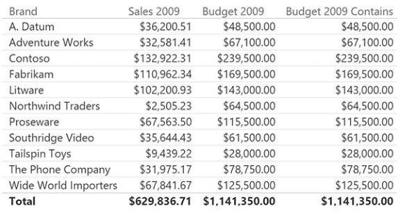
This code is much more complex than the simple INTERSECT used in the previous expression, but if you need to use such a pattern in Excel 2010 or Excel 2013, it is your best option. Figure 9-7 shows how the two measures return the very same number, even if they use a slightly different technique to obtain the result.
FIGURE 9-7 Budget 2009 and Budget 2009 Contains compute the very same result.
The technique discussed here does not require you to change the data model because it relies only on the use of DAX. It works just fine, but the code tends to be somewhat complex to write, especially if you are using an older version of Excel. With that said, the version using set functions might easily become too complex if, instead of only two, you start to have a significant number of attributes in the Budget table. In fact, you will need to add a new INTERSECT function call for each of the columns that define the granularity of the budget table.
Another issue with this measure is performance. The INTERSECT function will rely on the slower part of the DAX language, so for large models, performance might be suboptimal. Fortunately, in January 2017, DAX was extended with a specific function to handle these scenarios: TREATAS. In fact, with the latest versions of the DAX language, you can write the measure as follows:
Click here to view code image
Budget 2009 := CALCULATE (
SUM ( Budget[Budget] ),
TREATAS ( VALUES ( Budget[Brand] ), 'Product'[Br TREATAS ( VALUES ( Budget[CountryRegion] ), Stor
)
The TREATAS function works in a similar way to INTERSECT. It is faster than INTERSECT, but much slower than the relationship version we are about to show in the next section.
Filtering through relationships
In the previous section, we solved the scenario of budgeting by using DAX code. In this section, we will work on the same scenario, but instead of using DAX, we will solve it by changing the data model to rely on relationships that propagate the filter in the right way. The idea is to mix the first technique, which is the reduction of granularity of Sales and the creation of two new dimensions, with a snowflake model.
First, we can use the following DAX code to create two new dimensions: Brands and CountryRegions.
Click here to view code image
Brands =
DISTINCT ( UNION (
ALLNOBLANKROW ( Product[Brand] ), ALLNOBLANKROW ( Budget[Brand] )
)
)
CountryRegions = DISTINCT (
UNION (
ALLNOBLANKROW ( Store[CountryRegion] ), ALLNOBLANKROW ( Budget[CountryRegion] )
)
)
After the tables are created, you can set up the relationships by making them a
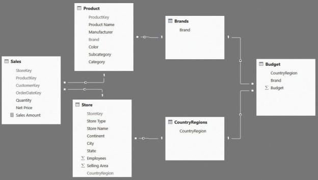
snowflake (for Sales) and direct dimensions (for Budget), as in the data model shown in Figure 9-8.
FIGURE 9-8 Brands and CountryRegions are additional dimensions that fix the granularity issue.
With this model in place, which is a perfect star schema, you can use the Brand column in Brands or the CountryRegion column in CountryRegions to slice both Sales and Budget at the same time. You need to be very careful to use the right column, however. If you use the Brand column in Product, it will not be able to slice Brands or, by extension, Budget, because of the direction of relationship cross-filtering. For this reason, it is a very good practice to hide the columns that filter the model in a partial (and unwanted) way. If you were to keep the previous model, then you should hide the CountryRegion column in both Budget and Store, as well as the Brand column in Product and Budget.
The good news is that, in Power BI, you have full control over the propagation of relationship cross-filtering. Thus, you can choose to enable bidirectional filtering on the relationship between Product, Brands, and CountryRegions. The model you obtain is shown in Figure 9-9.
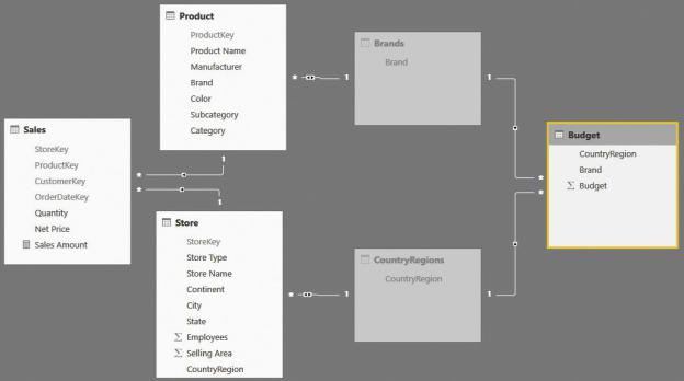
FIGURE 9-9 In this model, Brands and CountryRegions are hidden, and their relationships with Product and Store are set as bidirectional.
At first, there seems to be no difference between Figure 9-8 and Figure 9-9. But even if the models contain the very same tables, the difference is in how the relationships are set. The relationship between Product and Brands has a bidirectional filter, exactly like the one between Store and CountryRegions.
Moreover, both the Brands and CountryRegions tables are hidden. This is because they now became helper tables (that is, tables that are used in formulas and code but are not useful for the user to look at). After you filter the Brand column in Product, the bidirectional filter in the relationship moves the filter from Product to Brands. From there, the filter will flow naturally to Budget. The relationship between Store and CountryRegions exhibits the same behavior. Thus, you built a model where a filter on either Product or Store filters Budget, and because the two technical tables are hidden, the user will have a very natural approach to it.
This technique offers significant performance advantages. In fact, being based on relationships, it improves the use of the fastest part of the DAX engine, and it applies filters and uses filter propagation only when necessary. (This is not the case with the solution described in the previous section, where we used a FILTER function regardless of an existing selection on affected dimensions.) This results in optimal performance. Finally, because the granularity issue is