


Sales YTD :=
CALCULATE (
[Sales Amount],
DATESYTD ( 'Date'[Date] )
)
 Note
Note
This is true not just for YTD calculations. All time-intelligence metrics are much easier to write when you use a date dimension.
By using a date dimension, you achieve the following:
 You simplify the writing of measures.
 You obtain a central place to define all columns related to the time that you will need to build reports.
 You improve the performance of the queries.
 You create a model that is simpler to navigate.
These are the advantages, but what about the disadvantages? In this case, there are none. Always using a time dimension, yields only advantages. Get used to creating a calendar dimension every time you build a data model, and don’t fall into the trap of choosing the easy way of using calculated columns. If you do, you will regret that decision sooner rather than later.
Understanding automatic time dimensions
In Excel 2016 and in Power BI Desktop, Microsoft has built an automated system to work with time intelligence—although the two tools use different mechanisms. We discuss both in this section.
 Note
Note
As you will learn in this section, we discourage you from using either of these systems because they do not provide the necessary flexibility and ease of use that you need in your models.
Automatic time grouping in Excel
When you use a PivotTable on an Excel data model, adding a date column to the
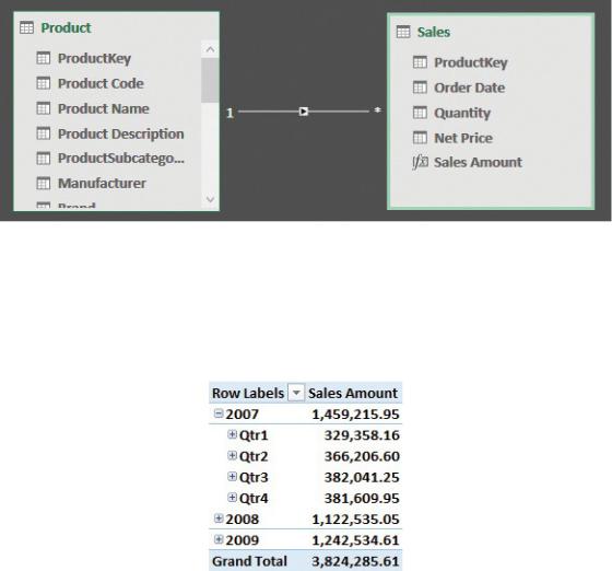
PivotTable prompts Excel to automatically generate a set of columns in the PivotTable to automate date calculations. For example, you might start with the model shown in Figure 4-5, where the Sales table contains only one date column, the Order Date column.
FIGURE 4-5 The Sales table contains a date column, which is Order Date, and no columns with the year and/or month.
If you create a PivotTable with Sales Amount in the values area and Order Date in the columns, you will notice a small delay. Then, surprisingly, instead of seeing the Order Date, you will see the PivotTable shown in Figure 4-6.
FIGURE 4-6 The PivotTable slices the date by year and quarter, even if you did not have those columns in the model.
To make this PivotTable slice by year, Excel automatically added some columns to the Sales table, which you can see if you reopen the data model. The result is shown in Figure 4-7, which highlights the new columns added by Excel.

FIGURE 4-7 The Sales table contains new columns, which were automatically created by Excel.
Notice that Excel did exactly what we suggested you avoid: It created a set of columns to perform the slicing directly in the table that contains the date column. If you perform the same operation on another fact table, you will obtain a new set of columns, and the two cannot be used to cross-filter the tables. Moreover, because the columns are created in the fact table, on large datasets, this takes time and space in the Excel file. You can find more information about this feature at https://blogs.office.com/2015/10/13/time-grouping-enhancements-in-excel- 2016/. This article also contains a link to a procedure that involves editing the registry to turn off this feature. Unless you work with very simple models, we recommend you follow the procedure to disable automatic time grouping and learn the correct way to handle it by hand, which we explain in this chapter.
Automatic time grouping in Power BI Desktop
Power BI Desktop tries to make time-intelligence calculations easier by automating some of the steps. Unfortunately, even if it automates the steps slightly better than Excel, Power BI Desktop is not the best solution for time intelligence.
If you use the same data model as in Figure 4-7 in Power BI Desktop and you build a matrix with the Order Date column, you obtain the visualization shown in Figure 4-8.