through a SQL view, or by using the query editor. Performing the same operation with DAX proves to be very complex, since DAX is not intended as a data manipulation language, but it is primarily a query language.

The good news is that, once the many-to-many is materialized, the formula becomes extremely simple to author because you only need to compute the sum of the hours multiplied by the percentage. As an additional option, you can also compute the hours multiplied by the percentage during extract, transform, load (ETL) to avoid the multiplication at query time.

Using the fact tables as a bridge

One curious aspect of many-to-many relationships is that they often appear where you don’t expect them. In fact, the main characteristic of many-to-many relationships is the bridge table, which is a table with two relationships in the opposite direction that link two dimensions. This schema is much more frequent than you might expect. In fact, it is present in any star schema. In Figure 8-20, for example, you can see one of the star schemas we have used multiple times in the demos for this book.

FIGURE 8-20 This figure shows a typical many-to-many relationship with the number of rows in each table.

At first sight, it looks like there is no many-to-many relationship in this model. However, if you carefully consider the nature of many-to-many relationships, you can see that the Sales table has multiple relationships in opposite directions, linking different dimensions. It has the same structure as a bridge table.

For all effects, a fact table can be considered as a bridge between any two dimensions. We have used this concept multiple times in this book, even if we did not clearly state that we were traversing a many-to-many relationship. However, as an example, if you think about counting the number of customers who bought a given product, you can do the following:

Enable bidirectional filtering on the relationship between Sales and Customer.

Use CROSSFILTER to enable the bidirectional relationship on demand. Use the bidirectional pattern with CALCULATE ( COUNTROWS ( Customer ), Sales ).

Any one of these three DAX patterns will provide the correct answer, which is that you filter a set of products, and you can count and/or list the customers who bought some of those articles. You might have recognized in the three patterns the same technique we have used to solve the many-to-many scenario.

In your data-modeling career, you will learn how to recognize these patterns in different models and start using the right technique. Many-to-many is a powerful modeling tool, and as you have seen in this short section, it appears in many different scenarios.

Performance considerations

Earlier, we discussed different ways to model complex many-to-many relationships. We concluded that if you need to perform complex filtering or multiplication by some allocation factors, then the best option, from both a performance and a complexity point of view, is to materialize the many-to-many relationship in the fact table.

Unfortunately, there is not enough space in this book for a detailed analysis of the performance of many-to-many relationships. Still, we want to share with you some basic considerations to give you a rough idea of the speed you might expect from a model containing many-to-many relationships.

Whenever you work with a many-to-many model, you have three kinds of tables: dimensions, fact tables, and bridge tables. To compute values through a many-to-many relationship, the engine needs to scan the bridge table using the dimension as a filter, and then, with the resulting rows, perform a scan of the fact table. Scanning the fact table might take some time, but it is not different from scanning it to compute a value when the dimension is directly linked to it. Thus, the additional effort required by the many-to-many relationship does not depend on the size of the fact table. A larger fact table slows down all the calculations;

many-to-many relationships are not different from other relationships.

The size of the dimension is typically not an issue unless it contains more than 1,000,000 rows, which is very unlikely for self-service BI solutions. Moreover, as already happened with the fact table, the engine needs to scan the dimension anyway, even if it is directly linked to the fact table. Thus, the second point is that the performance of many-to-many relationships does not depend on the size of the dimension linked to the table.

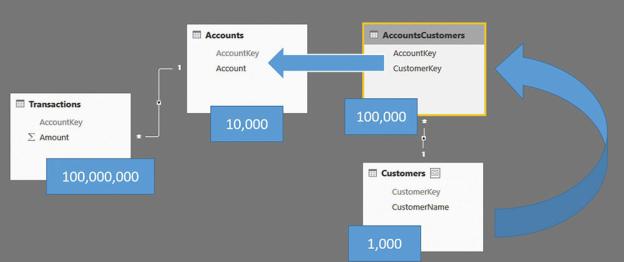
The last table to analyze is the bridge. The size of the bridge, unlike the other tables, matters. To be precise, it is not the actual size of the bridge table that matters, but the number of rows that are used to filter the fact tables. Let us use some extreme examples to clarify things. Suppose you have a dimension with 1,000 rows, a bridge with 100,000 rows, and 10,000 rows in the second dimension, as shown in Figure 8-21.

FIGURE 8-21 This figure shows a typical many-to-many relationship with the number of rows in each table.

As mentioned, the size of the fact table is not useful. It has 100,000,000 rows, but this should not be intimidating. What changes the performance is the selectivity of the bridge table over the Accounts table. If you are filtering 10 customers, the bridge filters only around 100 accounts. Thus, you have a fairly balanced distribution, and performance will be very good. Figure 8-22 shows this scenario.

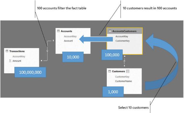
FIGURE 8-22 If the number of accounts filtered is small, performance is very good.

On the other hand, if the filtering of the bridge is much less selective, then performance will be worse depending on the number of resulting accounts. Figure 8-23 shows you an example where filtering 10 customers results in 10,000 accounts. In that case, performance will start to suffer.