

Photochemistry_of_Organic
.pdfProblems |
135 |
3.A plot of the inverse quantum yield for the photocycloaddition of 1-aminoanthraqui-
nones (AQ) and (E)-piperylene (Q) was found to be linear and the ratio of the slope, 0.20 dm3 mol 1, and intercept, 1.20, of this plot was equal to the Stern–Volmer constant for fluorescence quenching of AQ by Q, KSV ¼ 0.17 dm3 mol 1. It was concluded that the reaction proceeds from the excited singlet state of AQ via an exciplex intermediate 1ðAQ QÞ* . Explain. [Ref. 270]
4.The fluorescence quantum yield of anthracene in degassed acetonitrile is 0.3. It is reduced by 30% upon admission of air. Estimate the lifetime of the singlet state of anthracene in degassed solution and the rate constant of fluorescence. Refer to Section
2.2.1. The concentration of dioxygen in air-saturated acetonitrile is 2 10 3 M. [t0f ¼ 5:6 ns, kf ¼ 5.4 107 s 1]
5.Relative quantum yields F0/Fq have been measured as a function of quencher concentration, [q] ¼ 0., 0.02, 0.04, . . . , 0.2 M. The data, F0/Fq ¼ 1.0, 2.1, 3.2, 4.5, 4.8,
5.2, 6.0, 8.5, 8.5, 9.0, 9.0, obey a linear relationship (Equation 3.38), within experimental accuracy. Determine the intercept and the slope KSV (a) by linear regression and (b) by nonlinear least-squares fitting of the function log(Equation 3.38) to log(F0/Fq); cf. Figure 3.27. Which analysis is more reliable? [(a) intercept 1.40 0.33, slope 42 3; (b) intercept 1.08 0.10, slope 46 2]
6.Derive Equation 3.41.

4
Quantum Mechanical Models of
Electronic Excitation and Photochemical
Reactivity
4.1 Boiling Down the Schr€odinger Equation
The task of Þnding reasonably accurate solutions to Schr€odinger s Equation 1.5 for a medium-sized organic molecule looks like a mission impossible. For measure, consider a modestly sized molecule such as benzene that contains 42 electrons. A table listing only 10 values of its electronic wavefunction on a grid along each of its independent variables would contain 10126 entries (three coordinates must be speciÞed for each electron). This number is far larger than the number of atoms in the visible universe. Nevertheless, numerical solutions of the Schr€odinger Equation 1.5 can nowadays be obtained for reasonably large organic molecules with chemically useful accuracy using approximate ab initio or density functional theory methods.a
Trial wavefunctions are usually constructed by linear combination of Gaussian error functions that are convenient to integrate. The results can be of predictive value and such calculations have become everyday tools for chemists in all branches of chemistry, to guide experiments and not least to rule out untenable hypotheses. This is a remarkable achievement that seemed to be out of reach a few decades ago. Still, simple qualitative models that are amenable to perturbation theory are required to understand and predict trends in a series of related compounds. Our goal here is to describe the minimal quantum mechanical models that can still provide a useful qualitative description of electronically excited states, their electronic structure and their reactivity. Such models also provide a language to convey the results of state-of-the-art, but essentially Ôblack-boxÕ ab initio calculations.
a Closed, exact solutions of the Schr€odinger equation not being available for all except the most simple of systems, it is unavoidable to take recourse to approximations. The so-called ab initio methods refrain, however, from replacing parts of the calculations by empirical parameters that are optimized by adjustment to experimental data.
Photochemistry of Organic Compounds: From Concepts to Practice Petr Klán and Jakob Wirz © 2009 P. Klán and J. Wirz. ISBN: 978-1-405-19088-6
138 Quantum Mechanical Models
The electronic structure of molecules is commonly described in terms of molecular orbitals (MOs). This is a cavalier attitude because, strictly, orbitals cannot be used to describe many-electron systems. Atomic orbitals (AOs) are exact solutions of the Schr€odinger Equation 1.5 only for hydrogen-like atoms. If we attempt to construct an electronic wavefunction for, say, the helium atom by placing both electrons in the lowest
AO, f |
1s, |
which was determined |
for |
Heþ (a hydrogen-like atom), |
Cel |
(He) |
|
f |
|
(e |
) |
||
f |
|
2 |
|
|
|
|
|
1s |
1 |
|
|||
1sðe2Þ ¼ f1s, we run into two |
problems. The Þrst is that the Hamiltonian operator for |
||||||||||||
|
|
2 |
|
|
|
|
|
|
|
|
|||
helium contains the Coulomb term e |
/r12 accounting for the repulsion between the two |
||||||||||||
electrons. That term was not included in the determination of f1s for Heþ . If we calculate the lowest expectation value hE1i for the energy (Equation 1.14) of He using the AO obtained for Heþ , the resulting energy will be much too high, because the electrons are squeezed into the f1s orbitals of Heþ , which are too small. This can be amended by using some shielding factor that reduces the nuclear charge when determining AOs for He, a semiempirical procedure, or by re-optimizing the AO for He by taking account of electronic repulsion. Both procedures will make the AO for He more diffuse and thereby yield a lower expectation value hE1i.
Nevertheless, the calculated energy will still be substantially higher than that of the He atom in the ground state, unless we resort to an empirical shielding factor that is calibrated to yield the energy of He. This is due to a more fundamental and less tractable problem. By assuming that we can represent the electronic wavefunction for He by a product function of the type Cel(He) f1s(e1)f1s(e2), we implicitly assume that the motions of the two electrons are independent of each other: The square of such a wavefunction, which represents the time-averaged spatial distribution of the two electrons (Born interpretation, Section 1.4), is the product of their individual distributions, C2el f1sðe1Þ2f1sðe2Þ2. However, the combined probability of two events, such as that of throwing two ones with two dice, is equal to the product of the individual probabilities only if the two events are independent. This is clearly not the case for the movements of two electrons in an atom or molecule. Rather, given the position of one electron, it will be unlikely that the other electron is nearby. Electronic motions are correlated, electrons tend to avoid each other; if e1 happens to be on one side of the atom, the chances are that e2 will be on the other. The error associated with calculating time-averaged electrostatic interactions of electrons in stationary orbitals is called correlation error and amounts to about 1 eV (or 100 kJ mol 1) per electron pair in an organic molecule. Hence the energy calculated in this way will be too high, in accord with the variation theorem (Equation 1.14).
Keeping these cautionary remarks in mind, we nevertheless proceed to build trial wavefunctions for molecules as product functions of molecular orbitals. Moreover, we will construct the molecular orbitals as linear combinations of atomic orbitals (LCAOs), so that we can take advantage of the efÞcient RayleighÐRitz procedure (Equation 1.6). The idea behind the LCAO method is that electronic motion near a nucleus should be reasonably well described by an AO. Having committed all these sins, we will start by going one step further, namely by ignoring electronic interaction altogether. But do not despair! Although such crude methods can never give accurate energies for molecules and their excited states unless they are parameterized (semiempirical methods), they do retain a fair measure of physical reality, providing insight and allowing us to make useful predictions.
Before we proceed, recall the Aufbau principle: Having deÞned a set of orbitals for a given molecule, we Þll the electrons successively into the orbitals of lowest energy,
Boiling Down the Schrodinger€ Equation 139
allowing no more than two electrons of opposite spin per orbital. Why can we not place all the electrons into the lowest energy molecular orbital c1? This is a consequence of the Pauli principle (Equation 1.12), which demands a wavefunction to be antisymmetric with respect to electron exchange. Suppose the spin states of two electrons are the same, say aa (""). The spin function aa is symmetric (invariant to electron exchange), so the electronic wavefunction must be antisymmetric. A trial electronic wavefunction with both electrons in c1, C c1(e1)c1(e2) would be symmetric. We could construct an antisymmetric linear combination, C [c1(e1)c1(e2) c1(e2)c1(e1)], only to Þnd that this vanishes at all positions in space; no such state exists. Not so if the two orbitals carrying parallel spins are different: C [c1(e1) c2(e2) c1(e2)c2(e1)]/H2 is an acceptable antisymmetric wavefunction; it does change sign upon exchange of the two electrons.
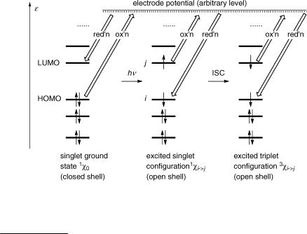
Provided that the electronic part of the wavefunction obeys the Aufbau principle, antisymmetric wavefunctions can always be constructed by using appropriate linear combinations (Slater determinants or antisymmetrized wavefunctions) and we can leave this technical problem to the computer programs. An occupation scheme deÞning the distribution of electrons among a set of given orbitals is called an electronic configuration.b The ground state of stable organic molecules will in general be represented by a closed-shell conÞguration, in which the lowest available orbitals are doubly occupied with electrons of antiparallel spin ("#) (Figure 4.1, left). We denote the wavefunction for a conÞguration by the letter x, that is, 1x0 ¼ c21c22 . . . c2i is the (singlet) ground-state conÞguration. Electronic excitation can then be described by raising one or more electrons from a bonding orbital
ci to an unoccupied orbital cj. The resulting (singlet or triplet) excited state conÞguration
becomes 1 or 3xi ! j ¼ 1 or 3ðc21c22 . . . cicj Þ.
Figure 4.1 Electronic configurations. The acronym HOMO designates the highest occupied MO and LUMO the lowest unoccupied MO of the ground state
b The expression conÞguration used in stereochemistry has a different meaning.

140 |
Quantum Mechanical Models |
In an excited, open-shell conÞguration, the Pauli exclusion principle allows us to have an excess of electrons with parallel spin (e.g. ## in the triplet state of Figure 4.1, right). In two conÞgurations with the same occupancy numbers but different total spin, the conÞguration with the highest spin will be the lowest in energy. In the present case, the triplet conÞguration will have a lower energy than the corresponding open-shell singlet. This is an extension of Hund s first rule, which was originally formulated for atoms. It is a rule, not a law, but it holds most of the time. Hund s rule may be attributed to the Fermi hole, the trafÞc law that keeps electrons apart in antisymmetric spatial wavefunctions (Figure 1.14). The energy difference between the singlet and triplet state is not manifested in Figure 4.1, because we have decided to ignore electronic interaction. It will show when we reintroduce it as an afterthought (Section 4.7).
Without even doing any MO calculation, we can already conclude from Figure 4.1 that any molecule M will become both a stronger oxidant and a stronger reductant upon electronic excitation. Ignoring entropy effects, the difference between the corresponding standard potentials E /V is equal to the excitation energy E0 0 of the excited singlet or triplet state measured in units of electronvolts (Equation 4.1). Thus, if the 0 0 band of S0 S1 absorption lies at 3 mm 1 (333 nm), both the oxidation and the reduction potential are shifted by 3.72 V! Note the change in sign in the second equation for oxidation.
E0ðM*=M .Þ E0ðM=M .Þ |
¼ |
E0 0ðMÞ |
¼ |
0:01036 |
E0 0ðMÞ |
1:240 |
~v0 0ðMÞ |
|||||
V |
|
|
eV |
|
|
kJ mol 1 ¼ |
|
mm 1 |
||||
E0ðM þ .=M*Þ E0ðM þ .=MÞ |
¼ |
E0 0ðMÞ |
¼ |
0:01036 |
E0 0ðMÞ |
1:240 |
~v0 0ðMÞ |
|||||
V |
eV |
|
|
kJ mol 1 |
¼ |
|
mm 1 |
|||||
Equation 4.1 Reduction and oxidation of excited molecules
4.2 Huckel€ Molecular Orbital Theory
H€uckel molecular orbital (HMO) theory271 deals only with the p-electrons of unsaturated systems; the s-electrons are considered to be part of a frozen core. That is, we use only the 2pz-AOs f on the unsaturated carbon atoms C1, C2, . . ., Cm, . . ., Cn, . . ., Cv, which are assumed to be orthonormal (orthogonal and normalized) (Equation 4.2).
< fmjfn> ¼ |
|
0 elsem ¼ n |
|
|
1 for |
Equation 4.2
The HMOs are constructed as linear combinations of the 2pz-AOs (LCAO):
v
X
c ¼ c1f1 þ c2f2 þ . . . þ cmfm þ . . . þ cnfn þ . . . þ cvfv ¼ Cmfm
m¼1
^ HMO
In order to Þnd solutions for the eigenvalue problem H c ¼ Ec, we have to set up the corresponding secular determinant (see Equation 1.16). No attempt is made to calculate the matrix elements of the secular determinant; instead, the matrix elements are
Huckel€ |
Molecular Orbital Theory |
141 |
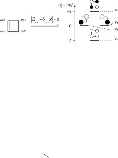
Figure 4.2 Huckel€ molecular orbitals for cyclobutadiene (3). The 2p-AOs are viewed from the top. The radius of the rings is proportional to the size of the AO coefficients |cjm|, so that their area is proportional to cjm2. The shading indicates the relative sign, i.e. white is used for cjm > 0 and black for cjm < 0 (or vice versa). The coefficients of the NBMOs c2 and c3 are |cjm| ¼ 1/H2 or 0 and those for c1 and c4 are |cjm| ¼ 0.5
treated as adjustable parameters (Equation 4.3). Thus the HMO model is devoid of any physical input; it makes use only of the topology (connectivity) of the p-system.
^ HMO |
jfm> ¼ aða constant value for carbon atoms CmÞ |
|||
Hmm ¼ < fmjH |
||||
Hmn ¼ < fmjH^ |
HMO |
jfn> ¼ |
b for m bound to n |
|
|
0 else |
|||
Equation 4.3 List of HMO matrix elements
The parameters a and b are called Coulomb integral and resonance integral, respectively. The resonance integral is a negative (stabilizing) energy. Now, let us set up the HMO secular determinant for cyclobuta-1,3-diene (3, Figure 4.2) as an example, using the matrix elements deÞned by Equation 4.3. The determinant contains the matrix elements Hmn dmn« with index m varying in the rows m ¼ 1, . . ., 4 and index n in the columns n ¼ 1, . . ., 4.
m
1
2 jjHmn dmn«jj ¼ 3
4
n |
1 |
2 |
3 |
4 |
a « b 0 b
|
b |
a « |
b |
« |
0 |
|
¼ |
0 |
0 |
b a |
|
b |
|
||||
|
|
|
|
|
|
|
|
|
|
|
|
|
|
|
|
|
|
b 0 b a «
Equation 4.4
A somewhat simpler form of the determinant is obtained by dividing all elements by b and substituting x for (a «)/b. Division by a constant is allowed, because the determinant is set equal to zero. We obtain the H€uckel determinant (Equation 4.5). All diagonal elements Bmm in the H€uckel determinant are equal to x and the off-diagonal elements Bmn are equal to zero, except for atoms m and n that are connected by a s-bond
¼ 1.
142 |
Quantum Mechanical Models |
x 1 0 1
|
|
|
|
|
|
|
|
1 |
x 1 |
|
0 |
|
|
|
|
jj |
Bmn |
|
dmnx |
jj ¼ |
|
x |
|
¼ |
0 |
||||||
|
|
|
0 |
1 |
|
1 |
|
||||||||
|
|
|
|
|
|
|
|
|
|
|
|
|
|
|
|
|
|
|
|
|
|
|
|
|
|
|
|
|
|
|
|
|
|
|
|
|
|
|
|
1 |
0 |
1 |
|
x |
|
|
|
|
|
|
|
|
|
|
|
|
|
|
|
||||
Equation 4.5 |
Huckel€ |
determinant for cyclobutadiene (3) |
|||||||||||||
|
|
|
|
|
|
|
|
|
|
|
|||||
Equation 4.5 is solved |
in a |
fraction of |
a second by a desktop computer using |
||||||||||||
a mathematical program such as MATLAB.c |
A set of four eigenvalues, «j ¼ a þ xj b, |
||||||||||||||
j ¼ 1, . . ., 4, is obtained, together with a set of four HMO coefÞcients, cj1, . . ., cj4, that is associated with each of the eigenvalues «j and deÞnes the four H€uckel molecular orbitals (Equation 4.6). The result is depicted graphically in Figure 4.2. The H€uckel calculation for 3 produces two nonbonding orbitals (NBMOs), «2 ¼ «3 ¼ a and x2 ¼ x3 ¼ 0.
v
X
cj ¼ cjmfm; j ¼ 1; 2; . . . n
m¼1
Equation 4.6 Huckel€ molecular orbitals (n ¼ v ¼ 4 for cyclobutadiene )
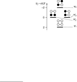
In general, any normalized linear combination of degenerate wavefunctions, wavefunctions that are associated with the same eigenvalue, is an equally valid
wavefunction. Thus, the orthogonal wavefunctions c02 and c03 shown in Figure 4.3, |
||||
p |
|
and c0 |
p |
shown in Figure 4.2. |
NBMOs, as are the |
c2 and c3 |
|||
c02 ¼ ðc2 þ c3Þ= |
2 |
3 ¼ ðc2 c3Þ= |
2 are equally acceptable solutions for the |
|
wavefunctions
Figure 4.3 Alternative set of HMOs for cyclobutadiene (3). The size of all coefficients is |cjm| ¼ 0.5
General solutions exist for the H€uckel determinants of special systems with any number n of carbon atoms, namely for the linear polyenes (Equation 4.7) and for the monocyclic systems (Equation 4.8).
«j ¼ a þ 2bcos |
p |
|
j ; j ¼ 1; 2; . . . ; n |
n þ |
1 |
Equation 4.7 General HMO energies for linear polyenes with n carbon atoms
c A simple HMO program is available on the Internet: http://www.chem.ucalgary.ca/SHMO/
Huckel€ Molecular Orbital Theory 143
2p
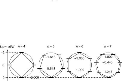
«j ¼ a þ 2bcos n j ; j ¼ 0; 1; 2; . . . ; n--1
Equation 4.8 General HMO solutions for monocyclic polyenes with n carbon atoms
From Equation 4.8, the energy of the lowest orbital is always «0 ¼ a þ 2b; that of the highest is a 2b if n is even. The other orbitals are twofold degenerate, «j ¼ «n j, because the cosine function is symmetric. Equation 4.8 can be recast graphically, by inscribing the n-polygon into a circle of radius 2b (Figure 4.4).
Figure 4.4 Frost–Musulin diagrams for the HMO energies of monocyclic systems
Systems such as cyclopentadienyl anion, benzene and tropylium cation with (4N þ 2) p-electrons (N ¼ 0, 1, 2, . . .) will thus have a closed shell, that is, four electrons in the degenerate pair of the highest occupied MOs in their ground conÞguration, and that is especially favourable energetically. This is the basis of the well-known H€uckel rule of aromaticity.
Having determined the HMO orbitals and Þlled in the appropriate number of p-electrons, we can characterize the resulting conÞguration by specifying the occupation number bj of each orbital cj; bj ¼ 2 for doubly occupied, bj ¼ 1 for singly occupied and bj ¼ 0 for unoccupied orbitals. The charge density qm of the p-electrons of that conÞguration on atom m is then given by Equation 4.9.
n |
|
qm ¼ Xj |
bj cj2m |
Equation 4.9 HMO charge density |
|
The bond order pmn between atoms m and n is given by Equation 4.10.
n |
|
pmn ¼ Xj |
bj cjmcjn |
Equation 4.10 HMO bond order
The bond order between bound pairs of atoms in cyclobutadiene (3) is 0.5 and the charge density equals unity on all atoms. On average there is exactly one p-electron on each carbon atom.

144 |
Quantum Mechanical Models |
4.3 HMO Perturbation Theory
HMO theory gives particularly simple and intuitively appealing results upon application of Rayleigh–Schr€odinger perturbation theory and we shall take advantage of this to interpret trends and make predictions (see, in particular, Section 4.6).d The equations for Þrstand second-order perturbation given below are derived in the Appendix (Section 4.11).
|
|
|
|
^ HMO |
of a perturbed system can be expressed as a sum of the |
|
|
The H€uckel operator H |
|||||
|
|
|
|
|
^ 0 |
^ |
operator of the parent molecule, H |
, and a perturbation operator, h (Equation 4.11). As for |
|||||
^ HMO |
|
|
|
|
^ |
|
H |
|
itself (Equation 4.3), we deÞne the perturbation operator h by a list of matrix |
||||
|
|
|
|
^ |
|
|
elements hmn ¼ < fmjhjfn>. |
|
|
||||
|
|
^ HMO |
^ 0 |
^ |
|
|
|
|
H |
¼ H |
þ h |
|
|
hmm ¼ dam½for inductive perturbationðsÞ at atomðsÞ m&
hmn ¼ hnm ¼ dbmn½for resonance perturbationðsÞ between atoms m and n& hmn ¼ hmm ¼ 0 otherwise
Equation 4.11 A list of suggested HMO perturbation parameters dam and dbmn for heteroatoms is given in Table 8.5
Changes in the resonance integrals between atoms m and n due to bond length alternation or twisted double bonds can be simulated using Equation 4.12.
bmn ¼ be Aðr r0Þ; A 0:02 pm 1; r0 ¼ 140 pm ðfor benzeneÞ bmn ¼ bcosðwÞ; where w is the angle of twist around the p-bond
Equation 4.12 Variation of bmn with bond length and twist 272
First-order perturbation uses the H€uckel orbital coefÞcients cjm of a given parent system to predict the shifts d«j on the corresponding orbital energies «j. The shift induced by an inductive perturbation dam is determined by the probability c2jm that an electron in orbital cj resides on atom m (Equation 4.13).
d«ðj 1Þ ¼ c2jmdam
Equation 4.13 First-order perturbation of the MO energy «j by an inductive effect dam introduced on atom m
An example of the inductive effect of 2-methyl substitution of buta-1,3-diene is shown in Figure 4.5. For reasons that will become clear shortly, the occupied orbitals are numbered 1, 2, . . . in order of decreasing energy and the unoccupied orbitals are numbered1, 2, . . . in order of increasing energy.
A change in the resonance integral between atoms m and n, dbmn, will change the energy
j by the amount given in Equation 4.14. For operators ^ that contain several elements 6¼0,
« h the first-order perturbations are additive.
d In the early days of quantum mechanics, perturbation theory was used mostly because it requires less computational effort than calculating each system separately. In the computer age, this is no longer a valid justiÞcation.

HMO Perturbation Theory |
145 |
Figure 4.5 Inductive effect |
of 2-methyl substitution of buta-1,3-diene using da2 |
(CH3) ¼ 0.4b. The numerical |
values of the HMO coefficients for butadiene are either |
|cjm| ¼ 0.372 or 0.602 |
|
d«ðj 1Þ ¼ 2cjmcjndbmn
Equation 4.14 First-order perturbation of the MO energy «j by a change in the resonance integral bmn by dbmn
An example of the conjugative effect of partial 1,4-bonding in cisoid butadiene is shown in Figure 4.6.
Figure 4.6 Conjugative effect of 1–4 interaction in cisoid buta-1,3-diene using db14 ¼ 0.3b
Perturbation theory gives reliable results only as long as the perturbation d«ðj 1Þ of a given orbital is small compared with the difference between its energy «j and that of all other orbital energies «i, j«j «ij d«ðj 1Þ. To account for perturbations on degenerate orbitals, «i ¼ «j, we need to solve the corresponding secular equation, that is, a 2 2 determinant for two degenerate MOs. But how small is small when «i 6¼«j? Moreover, is it justiÞable to use the HMO eigenfunctions of the parent system to calculate changes in the energies of the perturbed system? To answer these questions, we must go one step further and allow for variation in the wavefunctions upon perturbation. This requires some more work, but it will expose the limitations of Þrst-order perturbation theory. Being aware of these limitations, one can then in most, but not all, cases go back to use the simpler Þrst-order theory with conÞdence.
The energy shift of orbital cj calculated to second order is given by Equation 4.15. Second-
^ 6¼ order perturbations are not additive for operators h that contain several elements 0.