

Photochemistry_of_Organic
.pdf146 |
Quantum Mechanical Models |
|||||
|
n |
hcij |
^ |
c |
2 |
|
|
|
h |
|
|
||
|
d«jð2Þ ¼ d«jð1Þ þ Xi j |
|
j j i |
|
||
|
«j |
|
«i |
|||
|
6¼ |
|
|
|
|
|
|
Equation 4.15 Second-order perturbation of the MO energy «j |
|||||
|
^ |
|
are determined from the eigenfunc- |
|||
The perturbation matrix elements < cijhjcj > ¼ hij |
||||||
tions ci and cj of the unperturbed system, making use of the parameter list given in Equation 4.11 for the elements hmn in the AO basis. For example, for a single inductive perturbation at atom m, dam, we obtain hij ¼ hji ¼ cimcjmdam and for a single resonance
perturbation between |
atoms m and n, db |
mn, hij ¼ hji ¼ (cimcjn þ cjmcin)dbmn. If required, an |
||||||
1 |
|
|||||||
improved set of MOs cjð Þ |
for the perturbed system can be determined from Equation 4.16. |
|||||||
|
|
|
n |
|
^ |
|
2 |
|
|
|
|
|
hcij |
h c |
|
|
|
|
|
cjð1Þ ¼ cjð0Þ þ Xi j |
|
j j i |
|
cið0Þ |
||
|
|
«j |
|
«i |
|
|||
|
|
|
6¼ |
|
|
|
|
|
Equation 4.16 First-order perturbation of HMO wavefunctions
Let us look at a simple case to illustrate the predictions of Þrstand second-order perturbation and compare them with the full HMO calculation for the perturbed system. We choose ethylene as the parent system and look at inductive perturbation induced by introduction of a substituent at atom 1 or by replacing atom 1 by a heteroatom such N or O. The exact solution is obtained by solving the 2 2 secular determinant (Equation 4.17).
|
|
|
da |
1= |
b |
|
|
|
|
da |
|
|
|
|||
|
x |
|
|
1 |
|
|
|
|
|
|
||||||
1 |
þ |
|
|
|
|
x |
|
¼ x2 x |
|
b |
1 |
¼ 0 |
||||
|
|
da1=b |
|
|
|
|
2 |
|
4 |
|
|
|
||||
|
|
|
|
da1=b |
|
|
|
x |
a « b |
|||||||
x |
|
|
|
|
|
|
|
q |
|
|||||||
|
1;2 ¼ |
|
|
|
|
|
ð |
|
Þ þ |
|
; ¼ ð Þ= |
|||||
|
|
|
|
|
|
|
2 |
|
|
|
|
|||||
Equation 4.17 Exact HMO calculation for and inductively perturbed ethylene
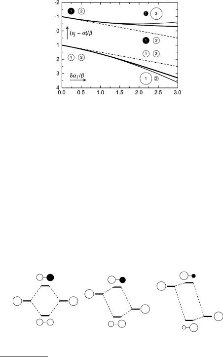
To illustrate the accuracy of Þrst- (Equation 4.13) and second-order (Equation 4.15) calculations, their results are compared with the exact solution (Equation 4.17) in Figure 4.7. The perturbation da1 is varied from 0 to 3b. The parameters for N (ethylenimine) and O (formaldehyde) are dam/b ¼ 0.5 and 1.0, respectively. If the term (dam/b)2 in the discriminant of Equation 4.17 is much smaller than 4 and can be neglected altogether, then Equation 4.17 is equal to the result of Þrst-order perturbation theory (Equation 4.13). If (dam/b)2 is smaller than 4 but non-negligible, the square root of Equation 4.17 can be expanded, (1 þ x)½ ¼ 1 þ 1/2x þ . . ., and we have the result of second-order perturbation (Equation 4.15). Thus, the results of Þrst-order perturbation are adequate for even a substantial perturbation such as the replacement of CH2 by O in formaldehyde.
However, it must be realized that this result is due to the large difference in energy
between the two HMOs of ethylene, « |
1 |
« 1 ¼ 2b. The criterion for a ÔsmallÕ |
perturbation |
||
|
|
2 |
|
||
hij now becomes clear: In the general case, Þrst-order perturbation is adequate for (d«i) |
|
/ |
|||
(«i «j)2 1 and second-order perturbation provided that (d«i)2/(«i «j)2 < 1. |
|
|
|||
Clearly, Þrst-order perturbation theory for degenerate orbitals cannot be done as described above, because the choice of any linear combination of degenerate
HMO Perturbation Theory |
147 |
Figure 4.7 Comparison of first- (dashed line), second-order (thin solid line) and full HMO calculations (thick solid line) for an inductive perturbation of ethylene. The radius of the circles indicates the size of the MO coefficients of c1 and c 1 on atoms 1 and 2, which remain unchanged upon first-order perturbation. The MOs obtained by second-order perturbation or by full HMO are concentrated more on the perturbed atom 1 in the bonding orbital c1
wavefunctions is arbitrary (cf. e.g. Figures 4.2 and 4.3). A secular determinant including both degenerate orbitals must be solved. This can be avoided if we select a basis set that is adapted to the reduced symmetry of the perturbed system so that the off-diagonal elements for the interaction between the two degenerate orbitals vanish. That may not be worth bothering with when computers do the job but, more important, the result becomes much more transparent when we start from symmetry-adapted orbitals. We will deal with symmetry considerations in the next section and postpone the discussion of Þrst-order perturbation of degenerate orbitals for now.
An important conclusion from perturbation theory is that the introduction of a resonance interaction will always destabilize the upper orbital and stabilize the lower one.e For a given size of the perturbation dbrs, the shifts decrease as the energy gap increases (Figure 4.8). Note that two basis AOs mix with equal weight when they are degenerate prior to interaction (left) and that the weight of the AO of the basis orbital with lower energy increases in the lower (bonding) MO as the energy gap between the basis orbitals increases (right).
Figure 4.8 Resonance interaction between two s basis AOs
e ÔBecause whoever has, to him will be given and he will have more; but from him who has not, even what he has will be taken away.Õ (Matthew 13 : 12).
148 Quantum Mechanical Models
4.4 Symmetry Considerations
Recommended textbooks.134,273Ð275
Symmetry considerations go a long way in predicting, inter alia, properties of wavefunctions, electronic states and transitions between molecular states. The mathematical treatment of symmetry operations is part of a special branch of mathematics known as group theory. Only a brief outline of some of its most important applications is given here.
A symmetry operation is a movement performed with a molecule Ð such as the reßection of its nuclear coordinates by a mirror plane s or rotation around an axis of symmetry C Ð that leaves the molecule unchanged. If a molecule is symmetrical, that is, if
|
|
|
^ |
|
|
||
it remains unchanged under some symmetry operation S, its molecular orbitals ci must be |
|||||||
^ |
ðciÞ ¼ ci, or |
2 |
^ |
ðciÞ ¼ ci |
|
^ |
|
either symmetric, S |
S |
, with respect to |
S, |
||||
|
antisymmetric, |
|
|||||
because the electronic distribution given by ci dv (Born interpretation, Figure 1.13) must |
|||
^ |
2 |
2 |
. For example, seven different symmetry operations can be |
remain unchanged, Sðci |
Þ ¼ ci |
||
performed on ethene (Figure 4.9). Group theory includes an eighth operation, the identity operation E; it does nothing, like the identity operation Ômultiplication by 1Õ in algebra. Any molecule or wavefunction will remain unchanged under the identity operation.
Figure 4.9 Symmetry operations
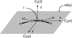
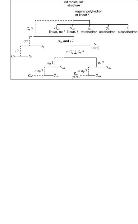
There are three twofold symmetry axes denoted C2(x), C2(y) and C2(z), which coincide with the coordinate axes x, y and z. The origin of the coordinate system shown in Figure 4.9 is an inversion centre i of the molecule, that is, the molecule remains unchanged when the nuclear coordinates of the atoms m, xm, ym and zm, are replaced by xm, ym andzm. Finally, there are three planes of symmetry, s(xy), s(xz) and s(yz), which coincide with the three planes spanned by a pair of coordinate axes [s(xy) is marked as a shaded plane]. Any molecule exhibiting the same set of symmetry operations belongs to the same point group, which is labelled by the Sch€onflies symbol D2h in the present case. The complete set of symmetry operations of an object deÞnes the point group, to which it belongs. A ßow chart to determine the point group of any molecule on the basis of its known (or assumed) 3D structure is shown in Figure 4.10. The combined operation of rotation and reßection through a plane perpendicular to an axis is an improper rotation; n- fold improper rotational axes are designated by the symbol Sn. Note that S1 s and S2 i.
The symbol s for symmetry planes is usually characterized by the index n (ÔverticalÕ, coincident with the rotational axis of highest order n) or d (ÔdihedralÕ or ÔdiagonalÕ, coincident with the rotational axis of highest order n and bisecting the angle between
Symmetry Considerations |
149 |
Figure 4.10 Flow chart for the determination of point groups (Schonflies€ symbols, n ¼ 2, 3, . . .). To find the point group of a given object, answer questions working downwards; follow the full line to the right if the answer is Yes or the dashed line to the left if it is No
orthogonal axes as in allene) and h (ÔhorizontalÕ, perpendicular to the rotational axis of highest order n).
The character table of a point group deÞnes the symmetry properties of a (wave) function as either 1 for symmetric or 1 for antisymmetric with respect to each symmetry operation.f The Þrst row lists all the symmetry operations of the point group and the Þrst column lists the Mulliken symbols of all possible irreducible representations, the symmetry transformation properties that are allowed for wavefunctions. As an
example, the character table for the D2h point group is given in Table 4.1. The character tables of all relevant point groups are given in many textbooks.134,273Ð275 The last
column shows the transformation properties of the axes x, y and z, which are used to determine electronic dipole and transition moments (Section 4.5).
Table 4.1 Character table for the point group D2h
D2h |
E |
C2(z) |
C2(y) |
C2(x) |
i |
s(xy) |
s(xz) |
s(yz) |
|
Ag |
1 |
1 |
1 |
1 |
1 |
1 |
1 |
1 |
|
B1g |
1 |
1 |
1 |
1 |
1 |
1 |
1 |
1 |
|
B2g |
1 |
1 |
1 |
1 |
1 |
1 |
1 |
1 |
|
B3g |
1 |
1 |
1 |
1 |
1 |
1 |
1 |
1 |
|
Au |
1 |
1 |
1 |
1 |
1 |
1 |
1 |
1 |
|
B1u |
1 |
1 |
1 |
1 |
1 |
1 |
1 |
1 |
z |
B2u |
1 |
1 |
1 |
1 |
1 |
1 |
1 |
1 |
y |
B3u |
1 |
1 |
1 |
1 |
1 |
1 |
1 |
1 |
x |
f Character tables of point groups of high symmetry (n > 2) have entries other than 1, but we need not deal with such groups here.
150 |
Quantum Mechanical Models |
We now return to first-order perturbation theory for degenerate orbitals (Section 4.3). As any linear combination of two degenerate orbitals ci and cj is equally valid, we set up a trial wavefunction function ck ¼ aki ci þ akj cj and we have to solve the secular Equation 4.18. The eigenvalues of the unperturbed system will be equal for all linear combinations,
«ið0Þ ¼ «jð0Þ ¼ «kð0Þ ¼ «ð0Þ. |
|
|
|
|
|
|
|
|
|
|
|
«ð0Þ þ d«kð1Þ « |
0 |
|
hkl |
1 |
|
« |
|
¼ |
0 |
|
hlk |
«ð Þ |
þ |
d«ð Þ |
|
|
|
|||
|
|
|
l |
|
|
|
|
|
||
|
|
|
|
|
|
|
|
|
|
|
|
|
|
|
|
|
|
|
|
|
|
Equation 4.18 First-order perturbation of two degenerate orbitals
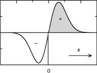
If we choose the linear combination of the degenerate orbitals such that one is symmetric and the other antisymmetric with respect to a symmetry element that is retained in the perturbed molecule, then the off-diagonal elements will vanish, hkl ¼ hlk ¼ 0, because integration of any function over the complete range of its variable x vanishes if the
Ð
function is antisymmetric: f(x)dx ¼ 0 (Figure 4.11). A function is said to be antisymmetric (a) if f( x) ¼ f(x). The product of two antisymmetric functions is symmetric (s); we write a a ¼ s; similarly, s s ¼ s but a s ¼ s a ¼ a.
Figure 4.11 Integral of an antisymmetric function
Having chosen a symmetry-adapted basis set ck and cl, the 2 2 determinant (Equation 4.18) is diagonal. The diagonal elements are the solutions, d«ð1Þ ¼ d«ðk1Þ and d«ðl 1Þ, with the associated symmetric and antisymmetric wavefunctions ck and cl. The Þrst-order perturbations of the energies «ðk0Þ and «l(0) are thus simply those given by the equations for Þrst-order perturbation of non-degenerate orbitals (Equations 4.13 and 4.14). The same result would have been obtained by solving the 2 2 non-diagonal determinant (Equation 4.18) obtained with any other linear combination. The equations for first-order perturbation can be applied to degenerate MOs of the parent system when the linear combination of the degenerate orbitals is chosen such that it is adapted to the symmetry of the perturbed system.
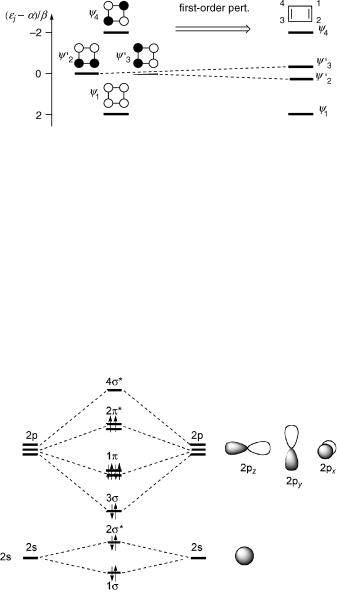
As an example, consider the effect of bond length alternation in cyclobutadiene (3). Let us assume that the molecule relaxes from a quadratic structure with an average bond length of 140 pm to one of the Kekule structures with the double bonds connecting, say, atoms 1Ð2 and 3Ð4 and that the length of the double bonds is reduced to 130 pm and that of the single bonds is increased to 150 pm. From Equation 4.12, we get b12 ¼ 1.22b and b23 ¼ 0.82b, that is, db12 ¼ db34 ¼ 0.22b and db23 ¼ db41 ¼ 0.18b. We choose the set of
Simple Quantum Chemical Models of Electronic Excitation |
151 |
Figure 4.12 Effect of bond length alternation in cyclobutadiene (3)
nonbonding orbitals c02 and c03 shown in Figure 4.12 (see also Figure 4.3), because these have the proper symmetry to deal with the perturbation. First-order perturbations are
additive; adding up the contributions (Equation 4.14) by each bond gives d«ðþ1Þ ¼ 0:40b and d«ð1Þ ¼ 0:40b.
Let us apply the same procedure to construct a qualitative MO diagram for the dioxygen molecule starting from the valence shell AOs of the separated O atoms, 2s, 2px, 2py and 2pz. The MOs are constructed by choosing symmetry-adapted linear combinations of the basis AOs, for example s ¼ (2s1 2s2)/H2, pz ¼ (2pz1 2pz2)/H2, and so on. The overlap between the 2pz orbitals is largest, leading to the large energy difference between the 3s and 4s MOs. The well-known diagram illustrated in Figure 4.13 results, showing that the HOMO 2p is twofold degenerate and holds only two electrons. Hence the ground state of dioxygen is a triplet state according to Hund s rule.
Figure 4.13 MO diagram for dioxygen
4.5 Simple Quantum Chemical Models of Electronic Excitation
Recommended textbook.15
Let us assume that organic molecules in their electronic ground state are reasonably well represented by a closed-shell electronic configuration built by Þlling electrons pairwise
152 |
Quantum Mechanical Models |
into the lowest energy HMOs in accord with the Pauli principle. Excited conÞgurations can then be constructed by promoting an electron to an unoccupied orbital (Figure 4.1). In terms of H€uckel theory, the excitation energy required to promote an electron from an orbital ci to an unoccupied orbital cj is equal to the difference of the corresponding orbital energies (Equation 4.19).
«j «i ¼ ðxj xiÞb ¼ hc~v
Equation 4.19 HMO excitation energy
Excitation from the HOMO (c1), the highest occupied molecular orbital, to the LUMO
(c 1), the lowest unoccupied molecular orbital, of buta-1,3-diene (Figure 4.5) requires1.236b (b is a negative energy). We can use this result to obtain a Þrst calibration of b. The
absorption maximum of the Þrst p,p transition of buta-1,3-diene lies at n~max ¼ 4.6 mm 1; hence Ðb/hc 3.7 mm 1.
To calculate the transition moment Mel,n ! m ¼ e<Cel,n|S ri|Cel,m> (Equation 2.17), we
represent the ground-state |
wavefunction Cel,n by the closed-shell conÞguration |
||||||||
x0 |
c2c2 |
. . . c2 . . . c |
2 |
and the |
excited-state |
wavefunction Cel,m by xi |
! |
j |
¼ |
2 ¼2 |
1 2 |
i |
HOMO |
|
|
|
|
||
c1c2 |
. . . ci . . . cj . Integration over the |
coordinates |
of those electrons that occupy |
the |
|||||
same orbital in x0 and xi ! j gives unity, <ci|ci> ¼ 1, so the transition moment simpliÞes to Mel,i ! j ¼ e<ci|S ri|cj>, which involves only the orbitals ci and cj that participate in the transition. The operator S ri ¼ S(xi, yi, zi) and the electronic transition moment Mel,i ! j are vector quantities; the coordinates xi, yi and zi deÞne the positions of the electrons ei. To obtain the individual components of the electronic transition moment vector (Equation 4.20), we must integrate the products ciucj ¼ ucicj, where u stands for x, y or z. The coordinates u themselves are antisymmetric, so that Mel,i ! j will vanish, unless the transition density cicj is itself antisymmetric with respect to one of the coordinates u.
Mel;i ! j ¼ eð < cijxjcj >; < cijyjcj >; < yijzjyj >Þ
Equation 4.20 Electronic transition moment for a one-electron transition ci ! cj
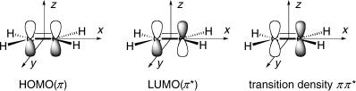
Consider the p,p transition of ethene. The HMOs of ethene are p ¼ (f1 þ f2)/H2 and p ¼ (f1 f2)/H2. The transition density, shown on the right-hand side of Figure 4.14, is the product pp* ¼1=2ðf1 þ f2Þðf1 f2Þ ¼1=2ðf21 f22Þ; this is easy to calculate, but the result is hard to swallow. Taken literally, it indicates a 50% chance that an electron is located in the left-hand pz-AO f1 and an equal chance that minus an electron is in the righthand pz-AO f2. Do not ask about the physical meaning of having Ôminus an electronÕ at
Figure 4.14 HMOs of ethene

Simple Quantum Chemical Models of Electronic Excitation |
153 |
some place in space! The transition density results from the quantum mechanical interference of two wavefunctions and has no meaningful classical analogy. The total charge is neutral, as it should be. The transition moment has a Þnite component in the x- direction, but vanishes in the y- and z-directions. Inserting the transition density into Equation 4.20 gives Mel,pp ¼ e[1/2(x1 x2), 0, 0], where x1 and x2 are the x-coordinates of the carbon atoms 1 and 2. With Equation 2.19, the oscillator strength is predicted to be f ¼ 0.3 for the p,p transition of ethene.
Symmetry considerations (Section 4.4) lead to the same conclusion. The transformation properties of the p- and p -orbitals of ethene are determined by inspection of Figure 4.14. All orbitals are symmetric (1) with respect to the identity operation. Under C2(z) the p-orbital is symmetric (1), the p -orbital is antisymmetric ( 1), and so on. This leads to the row vectors (1, 1, 1, 1, 1, 1, 1, 1) for the p-orbital and (1, 1, 1, 1, 1, 1, 1, 1) for the p -orbital. The p-orbital (Table 4.1) thus belongs to the irreducible representation B1u and the p -orbital to B2g. The vector obtained for the transition density pp (1, 1, 1, 1, 1, 1, 1, 1) belongs to the representation B3u, which transforms like the x-axis (see the last column of Table 4.1), indicating that the transition moment lies parallel to the x-axis. The above exercise may appear to be rather futile, given that we had arrived at the same conclusion by simple inspection of the HMO orbitals (Figure 4.14). Note, however, that symmetry arguments do not require any explicit calculation at all. The irreducible
representations, to which MOs constructed from a given set of basis orbitals must belong, can be determined from group theory alone.134,273,274,275 Electronic transitions whose
transition moment is zero in all directions because the transition density belongs to an irreducible representation that does not transform like any of the symmetry axes are said to be symmetry forbidden.
Is H€uckel theory any good at predicting absorption spectra and transition moments? The answer is a mixed bag: yes and no. To begin with, H€uckel theory is blind to the energy difference between singlet and triplet conÞgurations because it ignores electron repulsion altogether. Moreover, we shall see that for several classes of molecules the lowest excited singlet state is not adequately described by the lowest singly excited conÞguration. Consider the cyclic systems with (4N þ 2) p-electrons (N ¼ 1, 2, 3, . . .), which are particularly stable (ÔaromaticÕ) in the ground state (H€uckel rule, Section 4.2). HMO theory predicts that all four lowest-energy transitions in such systems have the same energy. In fact, these transitions are split into three absorption bands of substantially different energy in benzene (the Ôbenzene catastropheÕ) and two in cyclopentadienyl cation. Our goal is to understand where HMO theory works and when we need to upgrade the simple model (Section 4.7).
Let us take the good news Þrst. HMO performs fairly well in predicting the position and intensity of certain types of bands in many classes of compounds. From Equation 4.7, the HOMOÐLUMO energy gap of linear polyenes (ethene, buta-1,3-diene, hexa-1,3,5-triene,
. . .) can be expressed by Equation 4.21.g
«LUMO «HOMO ¼ 4bsin½p=ð2n þ 2Þ& 2bp=ðn þ 1Þ
Equation 4.21
g Recall that the index j of the LUMO is n/2 þ 1 and that of the HOMO is n/2. Moreover, cosa ¼ sin(a þ p/2), sina ¼ sin(p/ 2 a) and Þnally that sina a is a good approximation even for the smallest member, ethene, with n ¼ 2.
154 |
Quantum Mechanical Models |
The wavelength of a transition is directly proportional to the inverse of its transition energy; hence HMO theory predicts that the absorption wavelengths of linear polyenes are linearly related to the number of carbon atoms n (Equation 4.22).
n þ 1 l0--0 hc 2bp
Equation 4.22 HMO prediction for the wavelength of the HOMO–LUMO transition of linear polyenes
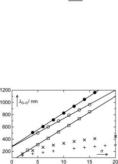
In Figure 4.15, the observed wavelengths l0–0 for eight all-trans linear polyenes276 ( ) are plotted versus n. Although l0–0 does increase with increasing length of the polyenes, the result is disappointing, because the observed relationship is clearly nonlinear; the absorption wavelengths reach a plateau for very long polyenes. Extrapolating linearly from the first three members of the series, we would predict that carrots are blue (b-carotene is an all-trans polyene with 11 conjugated double bonds).
Figure 4.15 Absorption bands of conjugated linear chains. The compound series are defined in the text together with the corresponding data sources
The deviations from Equation 4.22 can be traced to the alternation of bond lengths of linear polyenes. Even stronger effects of bond length alternation are evident in the series of polyacetylenes277 (þ ). We could use Equation 4.12 to adjust the resonance integrals b to the bond lengths of the essential single and double or triple bonds. Rather than introducing two new parameters using Equation 4.12 Ð which would Þx the problem Ð let us see whether the HMO prediction of Equation 4.22 works for linear conjugated systems that do not exhibit bond length alternation. Indeed it does. The symmetrical cyanines278 (&), which possess two equivalent resonance structures Me2NÐ(CH¼CH)(n/2Ð3) CH¼Nþ Me2
and Me2Nþ ¼(CH CH)(n/2Ð3)¼CH NMe2 and thus no alternating bond |
lengths, |
|||||
|
|
predicted linear relationship. The slope corresponds |
to |
b/ |
||
accurately obey the |
|
1 |
|
|
|
|
hc ¼ (3.05 0.05) mm |
|
. The Þrst absorption band of the linear chains HC2nHþ (radical |
||||
cations, .) and HC |
2nþ 1 |
Hþ (triplet ground state, *) and of the linear carbon chains C |
||||
|
|
241 |
n |
|||
(n ¼ odd, not shown) and Cn (n ¼ even, not shown) also increase linearly with n. |
|
|
||||
Systematic studies of the absorption spectra of benzenoid aromatic hydrocarbons, mostly done by Clar in the 1930s and 1940s,279 showed that these compounds exhibit four types of UVÐVIS absorption bands, which are shifted in a regular way along a homologous series such as the linear acenes (benzene, naphthalene, anthracene, . . .) (Figure 4.16).

Simple Quantum Chemical Models of Electronic Excitation |
155 |
Publisher's Note:
Permission to reproduce this image online was not granted by the copyright holder. Readers are kindly requested to refer to the printed version of this chapter.
Figure 4.16 Absorption spectra of the linear acenes280,281
Clar labelled the four bands a, p, b and b0 (in order of increasing energy for naphthalene, the b0 band of which is slightly above 5 mm 1) and empirically assigned them in well over 100 benzenoid hydrocarbons on the basis of their characteristics mentioned below and their regular shifts in homologous series. The a band is weak, log(«/ M 1 cm 1) 2Ð3, with sharp, irregular vibronic structure. Its position is insensitive to temperature, solvent polarity and polarizability. Its intensity, but not its position, increases strongly upon substitution, for example by halogens or alkyl groups. The p band is of moderate intensity, log(«/ M 1 cm 1) 4. It exhibits a distinct vibrational progression of 1400 cm 1 and is strongly red shifted in polar solvents and with increasing size of the hydrocarbon. The strong b band, log(«/M 1 cm 1) 5Ð6, is more diffuse and less sensitive to solvent and substitution. Finally, the b0 band, log(«/M 1 cm 1) 4Ð5, is less prominent and not always clearly discernible, because further transitions appear in the far-UV region. The a band is clearly seen as the Þrst absorption band of benzene and naphthalene, then hidden under the stronger p band in anthracene and tetracene, until it resurfaces, showing minute, relatively sharp features in the window between the p and the b band in pentacene and hexacene.
The p bands correlate well with HOMOÐLUMO energy gaps predicted by H€uckel theory (Equation 4.16) (Figure 4.17). Linear regression gives b/hc ¼ 2.2 0.1 mm 1. The points (*) for azulene (1) and cycl[3.3.3]azine (2) fall completely off the regression line (cf. Case Study 4.1). They are shown to emphasize that the correlation holds only for benzenoid hydrocarbons.
Excellent correlation was also found between Þrst ionization potential I1,v and the HOMO energies obtained by a slightly modiÞed H€uckel calculation for a large series of benzenoid hydrocarbons (Koopmans theorem, Section 4.7). The ionization potentials I1,v are also strongly correlated with the energies of the 1La bands, as would be expected on the basis of the pairing theorem (Section 4.6). A few outliers were noted, but a reinvestigation