

Photochemistry_of_Organic
.pdfQuantum Yields |
125 |
(penta-1,3-diene) is often referred to as a triplet quencher, because its triplet energy is well below that of most ketones, so that 3kq is close to diffusion controlled, whereas its singlet energy is usually higher than those of ketones, 1kq 3kq. Piperylene and other polyenes should always be freshly distilled because they form polymers that are poorly soluble, especially in polar solvents, giving turbid solutions. Sorbic acid or inorganic transition metal ions can serve as quenchers in aqueous solutions.
FC0=FCq ¼ 1 þ 3KSVcq
Equation 3.43 Stern–Volmer equation for the appearance of product C by the two-step reaction (Scheme 3.3) with quenching of only the triplet state
It is worth spending some time to digest the diagrams in Figure 3.26. Begin with the right-hand diagram, which represents the case of triplet quenching only. Consequently, the yield of product B that is formed directly from the singlet state is not affected by the quencher (dashed horizontal line). The straight line representing the formation of the triplet product C (dotted line, Equation 3.43) rises steeply because 3KSV is large. The solid line representing the disappearance of reagent A starts out with the same steep slope, but reaches a plateau at Fdis0=Fdisq ¼ 11 ¼ 1 þ a. At quencher concentrations cq > 0.2 M, the triplet reaction is completely suppressed, but the formation of the singlet product B remains unaffected. In the left-hand diagram, which displays quenching of both excited states, the dashed line representing the singlet product has a small slope corresponding to 1KSV. The dotted curve representing the formation of C looks the same as that on the righthand side, but is in fact no longer linear, showing upward curvature; at very high quencher concentrations it would rise quadratically, FC0=FCq ! 1KSV3KSVcq2 (Equation 3.42). Finally, the bent solid curve for Fdis0=Fdisq no longer saturates completely when the triplet pathway is suppressed, but continues to rise linearly with a slope of 1KSVð1 þ aÞ ¼ 55 M 1 above cq ¼ 0.1 M, as singlet quenching takes its toll.
Triplet sensitization (Section 2.2.2) can be used to determine 3KSV for the quenching of a triplet reactant. A complete reaction scheme for sensitization of a reactant A yielding product B from the triplet state would lead to a rather complex Stern–Volmer expression, if all steps are treated explicitly. However, if ISC of the sensitizer is very fast and efficient (FT ¼ 1) and if the concentration of A is chosen to be much higher than that of the quencher added, then we may assume that triplet energy transfer from the sensitizer to A is fast and efficient at all quencher concentrations, so that a plot of FB0=FBq versus cq will obey the simple Stern–Volmer relation and yield 3KSV as the slope.
A frequently encountered case is depicted in Scheme 3.4, where the singlet state of A, S1(A), reacts with a substrate B, for example an alkene yielding a cycloaddition product C. In most cases the substrate B will be in large excess, so that cB can be treated as a constant. Scheme 3.4 includes an intermediate A B that may represent an exciplex (Section 5.2) or a biradical intermediate (Section 5.4.4), which can proceed either to product C, A Bkr or
|
A··Bkd |
|
|
h |
S (A) + B |
1kBcB |
A··Bkr |
A + B |
1[A··B] |
C |
|
1kic + 1kf +1kisc |
1 |
|
|
|
|
|
Scheme 3.4 Bimolecular reaction
126 |
Techniques and Methods |
revert to the starting materials A þ B, A Bkd. All competing decay processes from S1(A) are assumed to lead back to the starting materials.
The quantum yield of product formation FC is equal to the product of the efficiencies of
the two reaction steps leading to C, FC ¼ 1hA B A BhC, where 1hA B ¼ 1kBcB= A BhC ¼ A Bkr=ðA Bkr þ A BkdÞ. The inverse of FC is then given
1=FC ¼ A BhC 1 þ |
1kB |
1t0cB |
||
1 |
|
|
1 |
|
Equation 3.44 Double reciprocal Stern–Volmer plot
Thus a plot of the inverse of FC versus the inverse of cB, a so-called double reciprocal plot, should be linear and the intercept/slope ratio gives 1KSV ¼ 1kB1t0 . See, however, the comments regarding statistical analysis given below.
The trapping of reactive intermediates such as carbenes or radicals by suitable additives may also reduce the quantum yield of product C. The Stern–Volmer treatment applies similarly and may be used to identify transient intermediates observed by flash photolysis; if half of the product is replaced by the trapping product, then the lifetime of the alleged reactive intermediate must be reduced by a factor of two at the same concentration of the trapping reagent.
Finally, a phenomenon called concentration quenching or static quenching can lead to upward curvature of Stern–Volmer plots even at moderate quencher concentrations (cq 0.01 M). Molecules that are located next to a quencher at the time of excitation will be quenched immediately. Therefore, the fluorescence decay curve will be nonexponential initially, exhibiting a very fast initial component. Moreover, the initial depletion of these molecules will result in an inhomogeneous distribution of the remaining excited molecules around the quenchers. As a result, the diffusion coefficient kd is no longer a constant, but becomes a function of time, kd(t), until the statistical distribution of excited molecules is re-established. The impact of these effects has been analysed in detail.231 Intrinsic rates of electron transfer in donor–acceptor contact pairs can be extracted from the resulting curvature in Stern–Volmer plots.232
A general remark regarding the statistical analysis of Stern–Volmer quenching data is in order. The standard errors of the measured quantum yield or lifetime ratios usually increase with increasing quencher concentration. One should either weight each data point by the inverse of its estimated variance or transform the appropriate Stern–Volmer equation to a form in which the distribution of standard errors is homoskedastic, that is, independent of the quencher concentration. The variance of the data points could be estimated from repeated measurements or from a priori considerations, but it is easier to fit the parameters of the appropriate homoskedastic function by nonlinear least-squares fitting (see Section 3.7.4). It is common, but bad, practice to transform Stern–Volmer relations to a linear but strongly heteroskedastic form and to analyse by linear regression without weighting.
In practice, the relative error of kobs ¼ 1/t and hence the error of logðkobsq=kobs0Þ is often independent of the quencher concentration. Consider, for example, triplet decay rate constants that were determined by flash photolysis in the absence, kobs0, and presence, q, of various quencher concentrations. We expect Equation 3.38 to hold,
Quantum Yields |
127 |
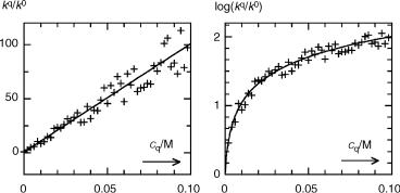
Figure 3.27 Heteroskedastic (left) and homoskedastic (right) Stern–Volmer plots
t0=tq ¼ kobsq=kobs0 ¼ 1 þ KSVcq. Figure 3.27 (left) shows artificial data that were generated by assuming KSV ¼ 1000 M 1 and adding 10% random noise to the values of kobs. The slope obtained by unweighted linear regression is KSV ¼ 965 43 M 1 and the intercept is ill-defined as 1.7 2.4. By taking the logarithm of the rate constants (righthand diagram), the same data become homoskedastic. Nonlinear least-squares fitting of the function log(a þ KSVcq) gives a much more accurate intercept, a ¼ 0.86 0.12, and a slope KSV ¼ 975 22 M 1. Usually one will have far fewer experimental data than are shown here, so one risks obtaining highly distorted results by linear regression. Having done the proper nonlinear analysis, one can still display the results as shown on the left to emphasize the linear relationship.
3.9.9Quantum Yields of Triplet Formation
The measurement of triplet quantum yields FT ¼ 1hISC is difficult because triplet states are transient intermediates. Phosphorescence quantum yields Fph represent a lower limit for
FT, because Fph ¼1hISC3hph, but the measurement of Fph requires low temperatures. Photothermal methods (Section 3.11) can be applied to the determination of triplet
quantum yields in solution when the triplet energy ET is known from phosphorescence measurements.233
|
Molar triplet–triplet absorption coefficients of some important triplet sensitizers with |
|||||||||
F |
T close to |
unity, |
such as |
benzophenone |
(« |
530 ¼ |
7200 M 1 cm 1) and xanthone |
|||
|
1 |
1 |
), have |
been determined |
|
|
234 |
so that monitoring triplet |
||
(«610 ¼ 5300 M cm |
|
reliably, |
|
|||||||
energy transfer by flash photolysis (Figure 2.18) can be used to estimate FT of other compounds. The triplet absorbance generated by sensitization is then compared with that observed by direct excitation of the probe.235 The concentrations of sensitizer and probe and of the excitation wavelength must be chosen such that the sensitizer absorbs most of the pump pulse in the energy transfer experiment. Alternatively, energy transfer to b-carotene (ET 96 kJ mol 1, «515 ¼ 187 000 M 1 cm 1) is very useful, not only to identify transient intermediates as triplets, but also to estimate FT.236 Although part of the excitation pulse is unavoidably absorbed by b-carotene, spontaneous ISC of b-carotene is inefficient on direct excitation. The near-IR emission of singlet oxygen has been applied to measure FT of Rose Bengal.237
128 |
Techniques and Methods |
Two self-calibrated methods are available that do not rely on the knowledge of FT of a reference compound. Horrocks et al. described an accurate method based on the measurement of triplet–triplet absorption by flash photolysis, in combination with Stern–Volmer analysis of fluorescence quenching (Section 3.9.8).238 Bromobenzene was used as a heavy-atom quencher of the fluorescence of 9-phenylanthracene. More recently, time-resolved measurements of delayed fluorescence (Section 2.2.4) were analysed to give accurate triplet quantum yields.239
3.9.10Experimental Arrangements for Quantum Yield Measurements
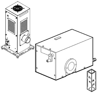
Whenever possible, essentially monochromatic light sources such as lowor mediumpressure mercury arcs equipped with bandpass filters or a monochromator (Figure 3.28), narrow-band photodiodes or lasers should be used for quantum yield determinations, because quantum yields can only be defined for monochromatic irradiation. This can be relaxed if the absorption spectrum of the actinometer is close to that of the sample (Section 3.9.6). One then assumes that the quantum yield is independent of the wavelength of irradiation. The stability of the light source over time is essential. Medium-pressure mercury arcs that have a stable output for many hours after a burn-in period of about 30 min are available. Xenon arcs tend to fluctuate abruptly when the arc between the electrodes jumps from one position to another. Intensity fluctuations of the light source in time can be monitored with photodiodes. This should be routinely done with pulsed lasers.
Figure 3.28 Components of an optical bench (source of radiation, monochromator, cuvette). Reproduced by permission of Newport Corp, Oriel Product Line
Quantum Yields |
129 |
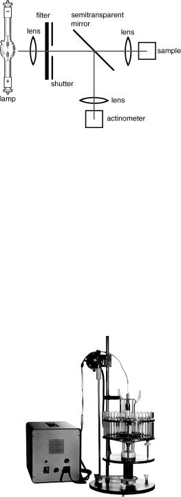
Figure 3.29 Experimental arrangement for measuring reaction quantum yields
Various arrangements are used for actinometry. In the setup shown in Figure 3.29, the sample and the actinometer are each placed in standard quartz cells (1 1 4 cm) that are equipped with a small magnetic stirring bar. Efficient stirring is essential when moderate absorbances, A < 2, are used. The sample and actinometer are irradiated simultaneously. First, the relative amount of light reaching the two cells from the beam splitter (a semitransparent mirror) is calibrated by placing an actinometer solution in both cells. Such a setup is insensitive to variations in the intensity of the light source. If the volumes of the sample and actinometer solutions are not the same, correction for volume V (c ¼ n/V) is required. For convenience, the actinometer may be replaced by a photodiode to monitor the relative light intensity continuously; the diode output is calibrated by placing the actinometer in the sample compartment. During subsequent irradiation of the sample, the amount of light is calculated from the diode reading.
A convenient, if somewhat less accurate, method for measuring a series of quantum yields of reaction is the merry-go-round setup (Figure 3.30). It holds about 20 sample and actinometer solutions with equal absorbance in cylindrical cells (test-tubes), which are
Figure 3.30 Merry-go-round apparatus. Reproduced by permission of Ace Glass Inc
130 |
Techniques and Methods |
rotated around a tubular light source such as a low-pressure mercury arc, a mediumpressure mercury arc equipped with appropriate filters or a fluorescent screen. Rotation ensures that all samples receive the same amount of incident light. After irradiation, the sample compositions are analysed using conventional methods such as NMR or GC. Caution is needed when the individual samples have different quantum yields, for example due to the addition of increasing amounts of quencher or reactant, because the amount of light absorbed by the reactant (Equation 3.18) will differ in the individual samples.
3.10 Low-Temperature Studies; Matrix Isolation
Recommended reviews.240–244
Studies involving the irradiation of solid solutions at low temperature have a long history, culminating in the identification of the triplet state of organic molecules by Lewis and Kasha in 1944.23 Ten years later, the expression matrix isolation was coined by George Pimentel,245 who pioneered the technique of co-condensing a substrate with a large excess of an inert gas on a cold surface, thus preventing any aggregation that may occur when a liquid is frozen. With the advent of commercial closed-cycle cryostats that obviate the need for liquid He and thus offer low-cost operation for matrix isolation in Ar (12 K) and in Ne (two-stage cooling, 4 K), the technique has found widespread use in many laboratories.
Nevertheless, the much less demanding method of cooling solutions in (mixtures of) organic solvents that freeze to solid, transparent glasses157,159 still has its place. Many
spectroscopic techniques are used to follow the reactions of matrix-isolated species, mostly IR (high-resolution spectra), optical spectroscopy and ESR, but also mass spectrometry of species that are released from the matrix by laser desorption or ion sputtering.246 A very powerful variant of matrix isolation is the deposition of mass-
selected ions.247
Many excellent reviews of matrix isolation work are available,240,242–244,247 and specific results are mentioned elsewhere in this text. In this section, we restrict ourselves to a few general remarks. Matrix isolation at low temperature mummifies highly reactive intermediates by two distinct effects and thereby permits their spectroscopic characterization without the need for fast detection. First, it isolates the reactive species in cages of an inert medium and thereby prevents diffusion and bimolecular reactions. Nevertheless, such reactions can be initiated at will, either by co-deposition with reactive gases such as dioxygen or carbon monoxide or by softening the matrix by a controlled rise in temperature. Second, monomolecular reactions are suppressed by the low temperature, ensuring that even small activation barriers become insurmountable and possibly by the cage effect inhibiting structural changes.
The reactive target molecules may be formed by rapid deposition of the gaseous eluates from flash vacuum pyrolysis, plasmas, and so on, or by irradiation of stable matrix-isolated molecules with high-energy radiation (UV, X-rays, g-rays, etc.). However, rare gas matrices are very poor at conducting heat. Consequently, any excess energy left in the primary products of a photoreaction will dissipate only slowly, allowing for further rearrangement. The same applies to hot molecules formed by internal conversion, so that the products formed by irradiation of matrix-isolated species
Photoacoustic Calorimetry |
131 |
may well result from hot ground-state reactions, which are rarely seen in solution (Section 2.3). Hence the counterintuitive finding that the product distributions formed by irradiation of molecules isolated in cold matrices may resemble those expected from high-temperature pyrolysis.
3.11 Photoacoustic Calorimetry
The measurement of heat deposition following the absorption of light can provide spectroscopic, kinetic and thermochemical information. The technique was invented in 1880 by Alexander Graham Bell as a means for the wireless transmission of speech.248 A membrane covered by a reflective coating transformed the sound waves of the speaker to an oscillating beam of reflected sunlight. The reflected beam was detected by the distant listener using a kind of stethoscope equipped with a closed transparent detector that was covered with black soot on the inside to reconstruct the sound wave pattern superimposed on the light beam. The oscillating release of heat developed by absorption of the light beam reproduced the sound wave as oscillating volume changes in the enclosed air.
Of course, Bell moved on to develop better methods of sound transmission, but thespectrophone was rediscovered some 80 years later and developed to a highly sensitive technique for trace gas analysis. As photochemists, we are more interested in the timeresolved analysis of heat deposition. A comprehensive review of the applications of photothermal methods in chemistry and biology covering the literature up to 1992 was published,249 and an excellent overview and discussion of the methodology appeared in 2003.250 The volume changes initiated in the solvent by the release of heat during photophysical and photochemical processes can be detected either with a microphone directly attached to the sample cell or optically by exploiting the resulting local changes in the refractive index of the solvent. Photorefractive techniques usually employ one of three methods, namely transient grating when two light waves with parallel polarization interfere, thermal lensing or beam deflection.
No attempt is made to analyse directly the complex but reproducible shock waves, which are produced by a short light pulse in the sample cell and recorded by a microphone. Rather, the shock waves produced in the sample are compared with those generated by a chromophore that is known to release the entire absorbed light energy as heat within a short time period (usually within 1 ns). This reference wave, produced for example by a solution of ferrocene, is called the T-wave. Delayed heat release in the sample due to the intervention of reactive intermediates is then reflected by a delay in the temporal evolution of the shock wave and incomplete heat release due to the formation of a (meta-)stable photoproduct or excited state of high energy is expressed in a diminution of the signal amplitude. The pair of signals is then analysed by mathematical deconvolution, which
amounts to an iterative fitting of the parameters of a (multi-)exponential decay function to reproduce the observed wave of the sample.251,252
For example, a solution of benzophenone in aerated acetonitrile releases part of the absorbed energy very rapidly (<1 ns) due to ISC and thermal relaxation, and the triplet state of benzophenone decays with a lifetime of about 200 ns. The observed signal then consists of a T-wave of reduced amplitude due to the fast process and the delayed heat
132 |
Techniques and Methods |
release due to the decay of the triplet state is modelled by adding small incremental T- waves for the heat released in short time intervals Dt as defined by the exponential decay function of the triplet state. The amplitudes and rate constant(s) of the processes occurring in the sample are then determined by iterative least-squares fitting of the nonlinear trial parameter(s) in the exponential function, the rate constant(s), to the observed sample signal (see Section 3.7.4 for the separation of linear and nonlinear parameters in leastsquares fitting).
Time-resolved photothermal methods are highly sensitive and cover a huge time range from about 1 ps to 1 s, although the individual methods are restricted to smaller time windows. They can detect reactive intermediates or conformational changes of enzymes that are invisible to other spectroscopic methods if these processes are accompanied by substantial enthalpic or volume changes. The techniques can be implemented at very little cost in any laboratory equipped with pulsed lasers and, when performed with due diligence, will yield highly accurate rate constants. In addition, they are unique in providing thermochemical data (heats of formation) of reactive intermediates.
However, reaction enthalpies obtained by photoacoustic methods must be considered with caution. Although the results are often highly reproducible, with standard errors of only a few kJ mol 1, the data may be fraught with hidden systematic errors, which arise mainly from two sources. First, the quantum yield of the process considered must be known with very high accuracy. This is a minor problem in the case of benzophenone considered above, because the triplet yield of benzophenone is known to be very close to unity. For intermediates formed with a smaller quantum yield, however, errors in the quantum yield of only a few percent translate to huge errors associated with the enthalpies of formation and decay of reactive intermediates. Second, the volume changes detected as pressure waves can be of thermal or non-thermal origin. Non-thermal volume changes can arise from Coulombic effects such as a change in the number of charges, dipole moments or hydrogen bonds associated with a reaction and from changes in the molar volume of the reactant associated with conformational changes or fragmentation reactions.
The separation of these cumulative effects is not an easy task, but is necessary for the determination of thermodynamic parameters, such as chemical bond strengths. Measuring very dilute water solutions at 3.9 C, where the thermal expansion coefficient of water vanishes (or at slightly lower temperatures in more concentrated aqueous solutions, such
as buffer solutions) can be used to separate the so-called structural volume changes from the thermal effects due to radiationless deactivation.253,254 In this way, it is also possible to
determine the entropy changes concomitant with the production or decay of relatively
short-lived species (e.g. triplet states), a unique possibility offered by these techniques.254,255
For reactions in organic solvents, the separation of the thermal and non-thermal effects is more complex. Some methods have been suggested.256 In view of the much larger value of the thermal expansion coefficient of organic solvents than the value for water, it is expected that the non-thermal volume changes in these solvents are in general much smaller than the thermal effects and can be neglected. However, caution is recommended, considering that some reactions (e.g. electron transfer reactions in polar organic solvents) might be accompanied by substantial solvent reorganization, which would give rise to large structural volume changes.

Single-Molecule Spectroscopy |
133 |
3.12 Two-Photon Absorption Spectroscopy
The interaction of a molecule with a strong laser pulse at a wavelength that is too long to populate an excited state by absorption of a single photon can lead to the simultaneous absorption of two or more photons. The phenomenon is described by nonlinear optics161 (Special Topic 3.1) and should be distinguished from the sequential absorption of two photons as, for example, in triplet–triplet absorption. Because the cross-sections for twophoton absorption are fairly small even under strong radiation, two-photon absorption is usually measured by fluorescence that is emitted well to the blue of the irradiation wavelength. Two-photon fluorescence excitation spectra differ from conventional absorption spectra because the selection rules for two-photon absorption are different. This permits the identification of excited states that have very low absorption coefficients.
Two-photon absorption is explored for applications in photodynamic therapy, for the release of photoremovable protecting groups (Special Topic 6.18) in living tissue and for stereolithography (3D optical storage). The strong light scattering by biological tissues hampers imaging by confocal microscopy. This is overcome by two-photon fluorescence microscopy because the scattering of near-IR radiation is low so that multiply scattered signal photons can be assigned to their origin allowing for deep-tissue imaging.257
3.13 Single-Molecule Spectroscopy
Recommended review articles.78,81,258–261
The detection and manipulation of single molecules became practicable only in the late 1970sj thanks to the combination of modern microscopic techniques and lasers and the impact of single-molecule spectroscopy (SMS) has grown tremendously over recent decades. The detection of single molecules is not primarily a sensitivity problem; photomultipliers have long been able to detect single photons that reach the photocathode. Rather, SMS is limited by background noise and by the photostability of the fluorescent molecules. Originally, SMS was possible only with a few highly photostable fluorescent molecules isolated in inert matrices at low temperatures. The implementation of clever techniques and statistical analyses to suppress stray light, noise and background signals now permits the detection of single molecules in biological media at room temperature. The signal-to-noise ratio was improved by orders of magnitude thanks to confocal microscopes that can probe sub-femtolitre volumes within biological tissue and discard adventitious light emerging from outside that volume.
Apart from the obvious challenge of reaching the ultimate limit of analytical chemistry, why is it of interest to detect single molecules? Conventional measurements done with an ensemble of molecules provide average values for the properties studied, but knowledge about the distribution of a property in time and space rather than its average value can be essential. Single-molecule detection provides information about the temporal fluctuation and local variation of these properties in heterogeneous media. Single molecules can act as
j . . . we never experiment with just one electron or atom or (small) molecule. In thought experiments we sometimes assume that we do; this invariably entails ridiculous consequences. . . E. Schr€odinger, Br. J. Philos. Sci. 1952, 3, 233–242.
134 |
Techniques and Methods |
highly sensitive reporters of their environment and movements. In a pioneering study, up to eight independent parameters (anisotropy, fluorescence lifetime, fluorescence intensity, time, excitation spectrum, fluorescence spectrum, fluorescence quantum yield, distance between fluorophores) of single molecules were simultaneously analysed, allowing for a quantitative analysis of 16 different compounds in a mixture via their characteristic patterns.262
Fluorescence correlation spectroscopy analyses the temporal fluctuations of the fluorescence intensity by means of an autocorrelation function from which translational and rotational diffusion coefficients, flow rates and rate constants of chemical processes of single molecules can be determined. For example, the dynamics of complex formation between b-cyclodextrin as a host for guest molecules was investigated with singlemolecule sensitivity, which revealed that the formation of an encounter complex is followed by a unimolecular inclusion reaction as the rate-limiting step.263
The ultimate goal in biological applications of single-molecule methods is to investigate biological processes in living organisms by tracking the movement of individual molecules in three dimensions and at molecular resolution. Examples of interest abound, such as protein folding and the invasion of a single cell by a virus and its attack on the cell s nucleus.264 SMS is able to detect rare events such as protein misfolding and reaction intermediates. The spatial resolution of modern optical imaging techniques is approaching 1 nm, far beyond the dispersion limit of a conventional microscope.265In situ dynamic studies of proteins (enzymes at work)83 and of intranucleosomal DNA have been reported.266
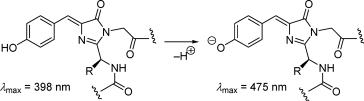
Green fluorescent protein (GFP) (Scheme 3.5) and its variants are particularly useful probes for live-cell imaging and to study intracellular dynamics.267,268 A Chemical
Abstracts search for GFP yielded about 35 000 references (June 2007), which appeared mostly during the last 15 years. SMS was used to explore the unfolding pathways of a green fluorescent protein (GFP) mutant called Citrine under nonequilibrium conditions.269 An intermediate on the unfolding/folding energy landscape was identified and two distinct conformations from which the protein unfolds along parallel pathways were found.
Scheme 3.5 The chromophore of green fluorescent protein (GFP)
3.14 Problems
1.Estimate the maximum amount of abiotic photoconversion in mol m 2 h 1 that can occur in surface waters in bright sunlight (800 W m 2). Assume that 5% of the solar
spectrum (Figure 1.1) is of sufficiently short wavelength to induce a photoreaction with a quantum yield of 1. [0.5 mol m 2 h 1]
2.Derive Equation 3.25 using the hint given in the footnote to that equation.