

Photochemistry_of_Organic
.pdf176 |
Quantum Mechanical Models |
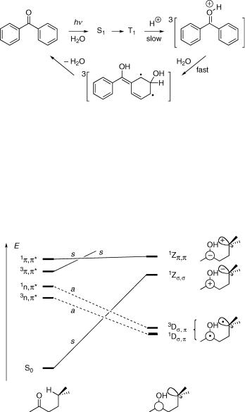
product that preserves one or more of the symmetry elements along the reaction coordinate. We can then connect states of the reactant and the product that belong to the same irreducible representation. We begin by estimating the energies of the lowest electronic states of the reactant and of the possible product(s). This information may be drawn from electronic spectra, calculations or educated guesswork. To be sure, the preferred reaction path may well be one not retaining any symmetry. We choose a symmetrical reaction path only because it allows us to construct a correlation diagram. Because potential energy surfaces are continuous, this path will give some indication of the shape of the surfaces nearby. Consider the protonation of a ketone in its lowest n,p excited triplet state (Figure 4.32). The carbonyl moiety is planar and we assume that the proton attacks the carbonyl oxygen in the plane of symmetry.
Figure 4.32 State-symmetry diagram for the protonation of an n,p excited triplet ketone
The n,p state of the ketone is strongly destabilized by protonation of the oxygen atom, so that it will have a higher energy than the p,p state in the conjugate acid. We can now classify the two lowest excited singlet states of reactant and product by simply counting the unpaired electrons. The wavefunctions of the closed-shell ground state and also those of the p,p excited states are symmetric (s), because they contain an even number of electrons in the antisymmetric (a) p and p orbitals (recall that a a ¼ s, Section 4.4). Those of the n,p states are antisymmetric (a) with respect to the plane of symmetry, because they have a singly occupied p -orbital and the n-orbital is symmetric, a s ¼ a. Connecting the states of the same symmetry, we see that the protonation of an n,p excited ketone is a state-symmetry forbidden reaction, as long as the plane of symmetry is retained.
Benzophenone is a very weak base in the ground state and its protonation requires very strong acid. The acidity of the conjugate acid, pKa(S0) ¼ 4.7, is, however reduced by four orders of magnitude in the excited triplet state pKa(S1) ¼ 0.4 (see also Case Study 5.1). Nevertheless, the protonation of triplet benzophenone is much slower than usual for an oxygen-protonation reaction, kHþ ¼ 3.8 108 M 1 s 1, and it is the rate-determining step preceding the faster hydration of the aromatic nucleus, k0 ¼ 1.5 109 s 1 (Scheme 4.4).332 The hydrated intermediate regenerates benzophenone after ISC and is responsible for the quenching of aromatic ketones by protons in aqueous acid reducing the quantum yields of their usual reactions. It does, however, open the way to some novel
Theoretical Models of Photoreactivity, Correlation Diagrams |
177 |
Scheme 4.4 Photohydration of benzophenone in aqueous acid
photoreactions333Ð335 of substituted aromatic ketones in aqueous acid (see also Scheme 6.239). The in-plane protonation of phenylnitrene is also state-symmetry forbidden (see Section 5.4.2).
A state-symmetry diagram for the Norrish type II reaction (Section 6.3.4) shows that it is allowed only from the n,p singlet and triplet states to give the covalent biradicals (Section 5.4.4) 1Ds;p and 3Ds;p, respectively, but not from p,p states (Figure 4.33).331
Figure 4.33 State-symmetry diagram for intramolecular hydrogen abstraction. The symmetry labels refer to the plane of the carbon chain
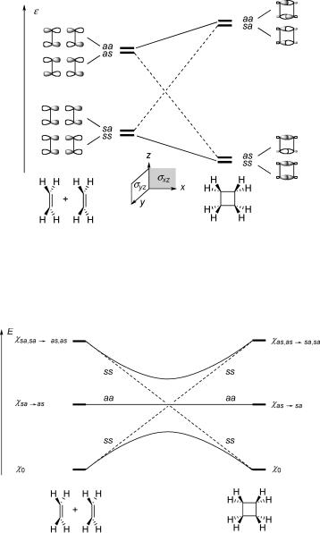
The orbital correlation diagrams put forth by Woodward and Hoffmann336 for electrocyclic and sigmatropic reactions (Section 6.1.2) and for cycloaddition reactions (Section 6.1.5) are well known and the details of their construction are not reiterated here. We show only the case of the [2s þ 2s] cycloaddition of two ethene molecules to cyclobutane as an example (Figure 4.34).
178 |
Quantum Mechanical Models |
Figure 4.34 Woodward–Hoffmann MO correlation diagram for [2 þ 2] cycloaddition. The labels s (symmetric) and a (antisymmetric) refer to the symmetry planes sxz and syz in that order
To predict the shape of potential energy surfaces along the symmetry-retaining reaction coordinate from an MO correlation diagram, one must construct a correlation diagram of the electronic conÞgurations (Figure 4.35).
Figure 4.35 Correlation diagram of the lowest configurations in [2 þ 2] cycloaddition
It is seen that the ground conÞguration of the two ethene molecules correlates with a doubly excited conÞguration of cyclobutane because the electron pair in the antisymmetric combination of the bonding p-orbitals of the ethenes (symmetry sa) is lifted to the antibonding s orbital of the same symmetry in cyclobutane. Starting from the singly excited conÞguration xsa ! as of symmetry aa, one ends up in the singly exited conÞguration
Problems |
179 |
of the same symmetry aa (dashed lines). ConÞguration interaction between x0 of symmetry ss and the doubly excited conÞguration of the same symmetry splits the two crossing states of symmetry ss apart (full lines), but a Ôsymmetry-imposedÕ barrier remains, which classiÞes the reaction as ÔforbiddenÕ in the ground state.
The reaction starting from the lowest singly excited state S1 (represented by the conÞguration xsa ! as in Figure 4.35) does not encounter a symmetry-imposed barrier, it classiÞes as ÔallowedÕ. In fact, reactions initiated from S1 usually do not proceed adiabatically to the lowest excited singlet state of the product. Rather, the region near the crossing of the Þrst-order diabatic PESs often represents a funnel, from where the molecule returns to the ground state PES. In short, ground-state reactions that are ÔforbiddenÕ by the WoodwardÐHoffman rules are generally ÔallowedÕ in photoreactions and vice versa, but exceptions from this general dichotomy do exist.337
Simple valence-bond theory provides another approach to construct correlation diagrams and to predict regions of diabatic surface crossings.20,338
4.10 Problems
1.Predict the effect of methyl substitution of azulene (replace C H by C Me individually in positions 1, 2, 4, 5 and 6) on the energy of the lowest excited state
S1. Use daC Me ¼ 0.333b to allow for the inductive (destabilizing) perturbation by the methyl group and compare with the experimental shifts of 790, 430, 370, 350 and 460 cm 1, respectively. [0.097, 0.033, 0.065, 0.034, 0.087b]
2.Predict the shifts of the Þrst absorption band of anthracene upon methyl substitution by inductive Þrst-order perturbation. [None]
3.Predict the shift of the Þrst absorption band of naphthalene radical cation upon 1- methyl substitution. [0.4252 ( 0.333)b ¼ Ð0.06b, hypsochromic shift, ref. 291]
4.Predict the effect of aza substitution on the Þrst absorption bands of naphthalene (quinoline and isoquinoline: energy, band intensity). [No shift, increased intensity of the 1La band, cf. Figure 4.27]
5.Predict the shifts of the Þrst ionization potential of naphthalene upon methyl
substitution in positions 1 and 2. The coefÞcients of the HOMO are cHOMO,1 ¼ 0.425 and cHOMO,2 ¼ Ð0.263. [Ref. 291]
6.Explain why the Þrst absorption band of cisoid dienes lies at longer wavelengths than that of transoid analogues. [Figure 4.6]
7.Verify the HOMOÐLUMO energy gaps calculated by PMO theory for the systems shown in Scheme 4.1.
8.Why are the absorption spectra of the radical cation and anion of anthracene nearly identical? [End of Section 4.7]
9.Calculate the transition moment and oscillator strength of the 1La transition of
naphthalene using the HMO coefÞcients given in Figure 4.26. [Mel,y ¼ 82 e pm, f ¼ 0.25].
10. Derive Equation 4.21 from Equation 4.7.
180 |
Quantum Mechanical Models |
11.Why do cross-conjugated alkenes absorb at shorter wavelengths than linearly conjugated alkenes? Compare hexa-1,3,5-triene and 1,1-divinylethene. [PMO]
4.11 Appendix
4.11.1First-Order Perturbation
Assume that the solution for the H€uckel secular determinant of a parent molecule has been determined, that is, that the eigenvalues «j and the associated set of orthonormal HMOs cj are known. We now introduce a ÔsmallÕ perturbation of the system, say by adding a substituent or by replacing one of the C atoms by a heteroatom, for example N. To this end, we must Þrst express the MO energies «j as a function of the MO coefÞcients. Inserting
|
|
|
|
^ |
|
|
|
|
|
|
|
Equation 4.6 into «j ¼ < cj jHjcj > we obtain Equation 4.38. |
|||||||||||
«j ¼ |
* v |
|
cjmfmjH^ j |
v |
cjnfn+ ¼ |
v v |
cjmcjnhfmjH^ jfni |
||||
|
X |
|
Xn 1 |
|
X X |
||||||
|
m |
¼ |
1 |
|
¼ |
|
m |
¼ |
1 n |
¼ |
1 |
|
|
|
|
|
|
|
|||||
Equation 4.38
The right-hand expression results from replacing the integral over sums by sums of
integrals. We replace the integrals < mj^ j n> by the parameter list (Equation 4.3), f
f H
retaining the atomic indices that assign the parameters to speciÞc atoms or bonds, because we will introduce perturbations at some particular atoms, am ¼ a þ dam, or bonds, bmn ¼ b þ dbmn:
v |
|
v |
|
v |
v |
|
v |
|
X |
X X |
X |
X |
|||||
«j ¼ cj2mam þ |
¼ |
|
cjmcjnbmn ¼ cj2mam þ 2 |
|
cjmcjnbmn |
|||
¼ |
|
|
m¼1 |
¼ |
|
n |
||
m |
1 |
m |
1 |
|
m |
1 |
m |
|
n6¼m
Equation 4.39
The last sum in Equation 4.39 runs only over pairs of atoms that are bound (m n),
because mn ¼ < mj^ j n> is zero otherwise, and is multiplied by two, because each bond b f H f
appears twice in the double sum on the left and bmn ¼ bnm. Introducing a perturbation at atom m, am ¼ a þ dam, the energy «j will change by d«j ¼ (q«j/dam)dam. The partial derivative of Equation 4.39 is (q«j/dam) ¼ cjm2, so that we obtain Equation 4.13 for the effect of an inductive perturbation dam on «j. Similarly, a change in the resonance integral between atoms m and n, dbmn, will change the energy «j by d«j ¼ (q«j/dbmn)dbmn. The partial derivative of Equation 4.39 with respect to bmn is (q«j/dbmn) ¼ 2cjmcjn (Equation 4.14).
4.11.2 Second-Order Perturbation |
|
|
|
|
|
^ |
^ 0 |
^ |
^ |
0 |
is the Huckel€ |
The operator of the perturbed system is written as H ¼ H |
þ h, where H |
|
|||
operator of the parent molecule and ^ the perturbation operator. We could, of course, set up h
a new H€uckel determinant for the perturbed system, but having the eigenvalues «jð0Þ and the |
|||
ð0Þ |
^ |
0 |
|
associated eigenfunctions cj |
with the operator H |
|
of the parent system at hand, we |
already have a good starting point for the new system. Therefore, the wavefunctions are set up as linear combinations of the functions cðj 0Þ (Equation 4.40).
Appendix |
181 |
n
c ¼ Xaj cðj 0Þ
j¼1
Equation 4.40
Optimized coefÞcients aj are determined by the variation method requiring the secular determinant to vanish. The indices of the columns and rows now refer to the basis set deÞned by Equation 4.40 and not to the AO basis as in Equation 4.5:
|
|
|
|
|
|
|
«1ð0Þ |
þ d«1ð1Þ « |
ð0Þ |
|
h12 ð1Þ |
|
|
|
. . . |
|
h1n |
|
|
|
|
|
|||
|
|
di |
|
|
|
|
|
|
h21 |
«2 |
þ |
d«2 |
|
« |
. . . |
|
h2n |
|
|
|
|
|
|||
Hij |
|
« |
|
|
|
|
|
: |
|
: |
|
|
. . . |
|
|
: |
|
|
|
|
0 |
||||
jj |
|
j |
|
jj ¼ |
|
|
|
|
|
|
|
|
|
|
|
|
|
|
¼ |
|
|||||
|
|
|
|
|
|
|
|
|
|
|
|
|
|
|
|
|
|
|
|
|
|||||
|
|
|
|
|
|
|
|
|
: |
|
|
|
: |
|
|
|
. . . |
|
|
: |
|
|
|
|
|
|
|
|
|
|
|
|
|
|
hn1 |
|
|
hn2 |
|
|
|
. . . |
0 |
|
1 |
|
« |
|
|
|
|
|
|
|
|
|
|
|
|
|
|
|
|
|
|
«nð Þ |
þ |
d«nð Þ |
|
|
|
|
|||||
|
|
|
|
|
|
|
|
|
|
|
|
|
|
|
|
|
|
|
|
|
|
|
|
||
|
|
|
|
|
|
|
|
|
|
Equation 4.41 |
|
|
|
|
|
|
|
|
|
|
|
||||
|
|
|
|
|
|
|
ð0Þ |
|
|
|
|
|
^ |
0 |
0 |
¼ 0, so that the off-diagonal |
|||||||||
The basis functions cj |
|
are eigenfunctions of H |
, Hij |
||||||||||||||||||||||
elements |
of |
the |
matrix |
Hij are equal to |
|
hij. In |
|
the diagonal |
elements |
we have |
|||||||||||||||
Hii « ¼ Hii0 þ hii « ¼ «ði 0Þ þ d«ði 1Þ «. Solving Equation 4.41 would provide the exact H€uckel eigenvalues of the perturbed system. Instead, we seek an approximation for the
Þrst eigenvalue, «1 «ð10Þ þ d«1. Based on the assumption that the perturbation is small
compared with the energy differences between «ð10Þ and the other eigenvalues of the unperturbed system, |«i(0) «1(0)| d«1 for i 6¼1, we can simplify Equation 4.41 as
follows. (i) For all diagonal elements except the Þrst, « «ði 0Þ. (ii) Only the off-diagonal
elements in the Þrst column and row affect «1 substantially; we set all others to 0. (iii) The |
||||||||||||||||||
Þrst-order perturbations d«ið1Þ |
are neglected in all diagonal elements except for i ¼ 1. |
|||||||||||||||||
Equation 4.42 is obtained. |
|
|
|
|
|
|
|
|
|
|
|
|
|
|
|
|||
|
«1ð0Þ |
þ d«1ð1Þ « |
0 h12 0 |
h13 |
|
. . . |
h1n |
|
|
|
|
|
||||||
|
|
h21 |
«2ð Þ |
|
«1ð Þ |
|
0 |
|
. . . |
|
0 |
|
|
|
|
|
|
|
|
|
h |
|
|
|
0 |
|
0 |
Þ . . . |
|
0 |
|
|
|
|
|
0 |
|
|
|
31 |
|
0 |
|
«ð Þ |
«ð |
|
|
|
|
|
¼ |
|||||
|
|
|
|
|
|
3 |
: |
1 |
|
|
|
|
|
|
|
|
||
|
|
: |
|
: |
|
|
|
. . . |
|
: |
|
|
|
|
|
|
||
|
|
h |
|
|
0 |
|
|
0 |
|
|
« 0 |
|
|
0 |
Þ |
|
|
|
|
|
n1 |
|
|
|
|
. . . |
|
«ð |
|
|
|
||||||
|
|
|
|
|
|
|
|
|
nð Þ |
|
|
1 |
|
|
|
|
||
|
|
|
|
|
|
|
|
|
|
|
|
|
|
|
|
|
|
|
|
|
|
|
|
|
|
|
|
|
|
|
|
|
|
|
|
|
|
Equation 4.42
A determinant does not change its value when a multiple of any row is added to an other row. Multiply the second row by h12=ð«ð20Þ «ð10ÞÞ and subtract the result from the Þrst. The
Þrst element becomes «01 þ d«ð11Þ « h12h21=ð«ð20Þ «ð10ÞÞ and the second element vanishes. Now multiply the third row by h13=ð«ð30Þ «ð10ÞÞ and subtract the result from the Þrst. The term h13 h31=ð«ð30Þ «ð10ÞÞ is subtracted from the Þrst element and the third element vanishes. Repeating up to the last row and evaluation of the diagonal determinant gives Equation 4.43.
«1 |
þ d«1 |
« |
0 |
|
ð0Þ!ð«2 «1 Þð«3 «1 Þ |
¼ |
|
|
ð0Þ |
ð1Þ |
n |
h1ihi1 |
ð0Þ ð0Þ ð0Þ ð0Þ . . . |
|
0 |
||
|
|
Xi 2 |
«ið Þ |
|
«1 |
|
|
|
|
|
¼ |
|
|
|
|
|
|
Equation 4.43
182 |
Quantum Mechanical Models |
We have assumed that «i(0) is not degenerate with any other eigenvalue «i(0) so that only the Þrst bracket can vanish and it will do so if
ð0Þ |
ð1Þ |
n |
h1ihi1 |
ð0Þ |
ð1Þ |
n |
h1ihi1 |
|||||
Xi 2 |
þ Xi 2 |
|||||||||||
« ¼ «1 |
þ d«1 |
|
|
|
¼ «1 |
þ d«1 |
|
|
|
|||
«ið0Þ |
|
«1ð0Þ |
«1ð0Þ |
|
«ið0Þ |
|||||||
|
|
¼ |
|
|
|
|
¼ |
|
|
|||
Equation 4.44
where the sum represents the second-order perturbation d«ð12Þ. The same can be done for any row i of Equation 4.42 to give the general equation for second-order perturbation (Equation 4.15), in which the upper indices (0) marking the eigenvalues «i of the unperturbed system have been dropped.

5
Photochemical Reaction Mechanisms
and Reaction Intermediates
5.1 What is a Reaction Mechanism?
The term reaction mechanism is part of the everyday language of chemists, yet it conveys different things to different people. The IUPAC Gold book (www.goldbook.iupac.org) defines the mechanism of a reaction as A detailed description of the process leading from the reactants to the products of a reaction, including a characterization as complete as possible of the composition, structure, energy and other properties of reaction intermediates, products and transition states. An acceptable mechanism of a specified reaction (and there may be a number of such alternative mechanisms not excluded by the evidence) must be consistent with the reaction stoichiometry, the rate law and with all other available experimental data, such as the stereochemical course of the reaction. On the basis of Occam s razor (Section 3.7.4), one should always choose the simplest mechanism that is consistent with all available evidence.
A truly mechanistic (in the sense of classical mechanics) description of a molecule s reaction is in fact prohibited by Heisenberg s uncertainty relations (Equation 2.1). Some reaction mechanisms of small molecules in the gas phase have been elucidated in the utmost detail, that is, reaction rate constants have been determined for individual rotational and vibrational quantum states of the reactant. We take a more modest view: a reaction mechanism is the step-by-step sequence of elementary processes and reaction intermediates by which overall chemical change occurs.
The mechanism of a photoreaction should ideally include a detailed characterization of the primary events as outlined by the classification of photochemical reaction pathways in Section 2.3; the lifetimes of the excited states that are involved in the reaction path, the quantum yields and hence the rate constants of all relevant photophysical and photochemical processes, in addition to the information about the structure and fate of any reactive intermediates, their lifetimes and reactivities.
Photochemistry of Organic Compounds: From Concepts to Practice Petr Klán and Jakob Wirz © 2009 P. Klán and J. Wirz. ISBN: 978-1-405-19088-6
184 |
Photochemical Reaction Mechanisms and Reaction Intermediates |
Knowledge of reaction mechanisms serves at least two purposes apart from the intellectual satisfaction of understanding . First, it provides a classification that reduces the myriad of chemical reactions of individual molecules to a more manageable set and thereby allows prediction by analogy. Second, it enables chemists to design reaction conditions in order to improve yields, the rate of product formation or selectivity of a reaction, to suppress undesired reactivity or to divert a reaction to form new products.
Before we proceed to discuss the properties of some of the most common reaction intermediates, we take a look at the simplest of elementary processes encountered in photochemistry: electron and proton transfer.
5.2 Electron Transfer
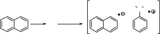
The redistribution of electrons associated with electronic excitation of a molecule changes all its physical properties, in particular its acidity (Section 5.3) and its redox properties. Electronically excited molecules are both strong oxidants and reductants (Section 4.1, Figure 4.1). Diffusional encounter of an excited molecule M with an electron donor D or acceptor A will therefore often result in the formation of a contact ion pair or solventseparated ion pair, depending on whether electron transfer occurs at a certain distance with at least one solvent molecule between M and D or A or only upon direct contact. For example, irradiation of naphthalene in an apolar solution containing N,N-dimethylaniline leads to the diffusion-controlled formation of a radical ion contact pair (Scheme 5.1).
The contact ion pair represents an excited supramolecular system called exciplex; its multiplicity will initially be that of its precursor contact pair and it has several options for further reaction. It could return to the ground state of the neutral reactants by radiative or nonradiative decay (return electron transfer, RET), it could undergo intersystem crossing,339 it could form a pair of free radical ions by escaping from the solvent cage340 or it could undergo some reaction such as proton transfer from D. þ to M. or rearrangement of D. þ to some product D0. þ .341 Its actual fate will depend strongly on solvent polarity and also on the presence of a magnetic field.339
The Coulombic attraction between two radical ions of opposite charge amounts to e2/ (4p«0«ra) in a solvent of relative static permittivity «r (formerly called dielectric constant), where «0 is the electric constant (also called permittivity of vacuum) and a is a parameter for the average distance between the centres of charge. In vacuum, the electrostatic work term to separate two singly charged ions is huge, e2/(4p«0«ra) ¼ 14.4 eV or 1.39 103 kJ mol 1 for a ¼ 100 pm («r ¼ 1), but it is strongly reduced in polar solvents. In water («r ¼ 78), it amounts to only 18 kJ mol 1, so that ion separation occurs on the time scale of nanoseconds.
|
|
Me N Me |
hν |
PhN(Me)2 |
.... |
|
S1 |
|
|
|
|
|
|
radical ion contact pair |
Scheme 5.1 Electron transfer

Electron Transfer |
185 |
The Gibbs free energy of photoinduced electron transfer, DetG , in an excited encounter complex (D A) can be estimated from Equation 5.1, where E (D. þ /D) is the standard electrode potential of the donor radical cation, E (A/A. ) that of the acceptor A and DE0–0 is the 0–00 excitation energy of the excited molecule (D or A ) that participates in the reaction.
DetG ¼ NAfe½E ðD. þ=DÞ E ðA=A. Þ& þ wðD. þ ; A. Þ wðD; AÞg DE0 0
Equation 5.1 Free energy of photoinduced electron transfer
In the general case, the electrostatic work terms w that account for the Coulombic attraction of reactants (D, A) and products (D þ , A ) are w(D, A) ¼ zDzAe2/(4p«0«ra) and w(D þ , A ) ¼ zD þ zA e2/(4p«0«ra), where zD and zA are the charge numbers of donor D and acceptor A prior to electron transfer and zD þ and zA are those after electron transfer. For neutral species D and A, zD ¼ zA ¼ 0. Choosing convenient units and collecting the constants we obtain the scaled Equation 5.2.
DetG |
|
|
96:49 |
E ðD. þ =DÞ E ðA=A. Þ |
þ |
138:9 |
zD þ zA zDzA |
|
119:6 |
DE0 0 |
||||
|
1 ¼ |
V |
|
|||||||||||
kJ mol |
|
« |
a=nm |
|
m |
m |
|
1 |
||||||
|
|
|
|
|
|
r |
|
|
|
|
|
|||
Equation 5.2 Scaled equation for the free energy of electron transfer
Mixing electron donor and acceptor molecules in apolar solution may be accompanied by the formation of weakly associated charge-transfer or electron-donor–acceptor(EDA) complexes in the ground state.342 In a simple quantum mechanical treatment, the groundstate wavefunction of EDA complexes may be described as a resonance hybrid of a no-bond ground state (A D) and a charge-transfer state (A D þ ) (Equation 5.3), where
c0,no bond 1 and c0,dative 0.
C0 ¼ c0;no bondCðA DÞ þ c0;dativeCðA D þ Þ
Equation 5.3 Wavefunction of an EDA ground state complex
The charge-transfer excited state is then represented by Equation 5.4, with c1,no bond 0
and c1,dative 1.
C1 ¼ c1;no bondCðA DÞ þ c1;dativeCðA D þ Þ
Equation 5.4 Wavefunction of an excited charge-transfer state
These wavefunctions account for the attractive force between A and D leading to the formation of an EDA complex, for its increased polar character and also for the existence of charge-transfer absorption that is often observed when EDA complexes form. Lowlying excited states of A or D þ must be included in the wave function to describe additional charge-transfer bands. These bands appear in addition to the absorption bands of the molecules A and D; they are usually broad and of low oscillator strengths because there is little overlap between the HOMO of the donor and the LUMO of the acceptor (Section 4.4, Equation 4.20). Many examples of the formation of EDA complexes between, for example, tetracyanoethylene and aromatic hydrocarbons are known. The