

Photochemistry_of_Organic
.pdfQuantum Yields |
115 |
Figure 3.25 Spectrophotometric observation of a photoreaction A ! B. The wavelengths of irradiation and of observation are designated lirr and l, respectively
solution of volume V to a constant photon flux q0 |
(Equation 3.16). The product of q0 |
m;p |
m;p |
and exposure time t is equal to the amount of photons that have impinged on the sample cell at time t. Note the distinction between the wavelength of irradiation, lirr, and the wavelengths of observation, l, which in most cases will not be the same. To simplify the notation, we will abbreviate absorbances A(l,t) at the wavelength of observation by At and those at the wavelength of irradiation, A(lirr,t), by At0. Replacement of the index t by 0 or ¥ indicates no and exhaustive irradiation, respectively. Similarly, absorption coefficients « and «0 refer to the wavelengths of observation and irradiation, respectively.
In order to determine the quantum yield F A ¼ dnA/dnp by absorption measurements, the molar absorption coefficients of the starting material A and of the product (mixture) B must be known. The differential amount of light absorbed by the reactant, dnp, during an exposure interval, dt, is then given by Equation 3.18. Replacing the partial absorbance by the reactant A at time t, A0A,t, by «0AnA(t)l/V, where l is the optical pathlength, we obtain
dn |
p ¼ |
q0 |
ð |
1 |
|
10 At |
0 |
Þ |
«0AnAðtÞl |
dt |
|
m;p |
|
|
|
VAt0 |
|||||
Equation 3.19
The total absorbance at the observation wavelength l is given by At ¼ [«AcA(t) þ «BcB(t)]l. With c ¼ n/V and nB(t) ¼ nA(t ¼ 0) nA(t), we can express the amount of component A in the solution as a function of the observed absorbance:
n |
t |
At A¥ |
V |
||
|
Að Þ ¼ lð«A «BÞ |
|
|||
|
|
Equation 3.20 |
|
||
The differential of Equation 3.20 is |
dnA ¼ dAV/([«A «B]l) and substitution using |
||||
Equation 3.20 gives Equation 3.21: |
|
|
|
|
|
|
dn |
|
nAðtÞ |
dA |
|
|
|
A ¼ At A¥ |
|
||
Equation 3.21

116 |
Techniques and Methods |
We insert Equations 3.19 and 3.21 into F A ¼ dnA/dnp and replace F A«A0 by Q(lirr) to obtain Equation 3.22, the general differential equation used for the spectrophotometric determination of quantum yields; the reason for introducing the so-called pseudo quantum yield Q ¼ F–A«A0 will become evident in Section 3.9.4.
l VAt0 l
Qð irrÞdt ¼ lq0 ; ð1 10At0 ÞðAt A¥Þ dAð Þ
m p
Equation 3.22 Differential equation for the spectrophotometric determination of quantum yields.
Approximate integration of Equation 3.22 is possible by linear interpolation of the reciprocal photokinetic factor,222 F(lirr,t) (Equation 3.23).
|
F |
ðlirr |
; t |
Þ ¼ |
|
ð1 10 A0t Þ |
; |
|
F |
ðlirrÞ ¼ |
Fðlirr; t2Þ þ Fðlirr; t1Þ |
|
|||||||||||||||
|
At0 |
|
|
|
|
||||||||||||||||||||||
|
|
|
|
|
|
|
|
|
|
|
|
2 |
|
|
|
|
|
|
|
||||||||
|
|
|
|
|
|
|
|
|
Equation 3.23 |
|
|
|
|
|
|
|
|
|
|
|
|
||||||
Integration of1Equation 3.22 for a short |
irradiation interval |
D |
t |
¼ |
t |
2 |
t |
, having replaced |
|||||||||||||||||||
|
1 |
|
|
|
|
|
|
1 |
|
|
|||||||||||||||||
the variable F |
|
(lirr,t) with the constant |
|
ðlirrÞ, gives the operational Equation 3.24, |
|||||||||||||||||||||||
|
F |
|
|
||||||||||||||||||||||||
which is generally applicable. |
|
|
|
|
|
|
|
ln At1 A¥ |
|
|
|
|
|
||||||||||||||
|
|
|
|
|
QðlirrÞ lq0 |
F |
|
V |
|
t t |
|
|
|
|
|
|
|||||||||||
|
|
|
|
|
|
|
|
|
|
|
|
|
|
|
A |
|
A |
|
|
|
|
|
|
|
|||
|
|
|
|
|
|
|
|
m;p |
|
ðlirrÞð 2 1Þ |
|
t2 |
|
¥ |
|
|
|
|
|
|
|||||||
Equation 3.24
When the absorbance at the irradiation wavelength is very large (total absorbance
At0 |
|
|
g |
|
|
|
1, then F |
ðl |
|
Þ |
|
|
|
ð |
|
|
1 |
þ |
|
|
2 |
Þ |
|
||||
> 3), so that 1 |
|
10 AðlirrÞ |
|
|
irr |
|
can be replaced by |
|
1=At |
0 |
|
1=At |
0 |
|
=2. |
||||||||||||
Exact integration |
|
of Equation 3.22 is possible when the reactant A can be irradiated at |
|||||||||||||||||||||||||
a wavelength where product B does not absorb, «B0 ¼ 0, yielding Equation 3.25: |
|
|
|||||||||||||||||||||||||
|
Q |
|
|
|
|
10At |
0 |
1 |
; where |
A |
0 |
A |
A |
«A0 |
|
|
|
|
|
||||||||
|
|
|
|
|
|
Vlog |
10A0 |
0 |
1 |
|
|
|
|
|
|
|
|
|
|
|
|
|
|
|
|
|
|
|
|
ðlirrÞ ¼ |
|
|
|
|
|
|
|
|
t or 0 |
¼ ð t or 0 ¥Þ |
|
|
|
|
|
|
|
|
|||||||
|
|
ltqm0 ;p |
|
|
|
|
|
|
|
«A «B |
|
|
|
|
|||||||||||||
Equation 3.25
When the reaction is monitored at the wavelength of irradiation, l ¼ lirr, then At or 00 in Equation 3.25 is the same as At or 0.
Prior to collecting accurate experimental data for spectrophotometric quantum yield determinations, one should always do a quick-and-dirty test run and decide which case is applicable (Equation 3.24 or 3.25). Note that in these equations the right-hand side must be multiplied by 1000 if the conventional but non-SI units [V] ¼ cm3, [«] ¼ mol 1 dm3 cm 1 and [l] ¼ cm are used. For quantitative work, it will be worthwhile to write a small program that computes the quantum yield from the measured absorbances according to the appropriate equation.
g Use the integral Ð(1/[a þ bepx])dx ¼ x/a ln(a þ bepx)/(ap), with x ¼ (At A¥), a ¼ 1, b ¼ 1 and p ¼ ln(10)«A0/(«A «B).
Quantum Yields |
117 |
3.9.4Reversible Photoreactions
In a reversible photoreaction (Scheme 3.2), such as the photoisomerization of azobenzene (Section 6.4.1), the differential rate for the disappearance of the reactant A is given by Equation 3.26, where dnp,A and dnp,B are the amounts of light absorbed by A and B, respectively, as defined by Equation 3.19.
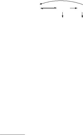
h
A  B
B
h
Scheme 3.2
dnA ¼ FA ! BðlirrÞdnp;A FB ! AðlirrÞdnp;B
Equation 3.26
Once a photostationary state (PSS) is reached upon irradiation at the wavelength lirr, the amount of reactant A no longer changes, dnA/dt ¼ 0, and by inserting Equation 3.19 for dnp,A and dnp,B we obtain Equation 3.27:
FA ! B ¼ «B0nBð¥Þ
FB ! A «A0nAð¥Þ
Equation 3.27
where nA(¥) and nB(¥) are the amounts of A and B present in the photostationary state and the absorption coefficients «0 refer to the wavelength lirr.
Hence the composition of the photostationary state, nA(¥)/nB(¥), is defined by the ratio of the quantum yields for the forward and backward reactions and that of the absorption coefficients «0. For a spectrophotometric determination of that composition, the absorption spectrum of at least one of the compounds A or B must be known. To determine the individual quantum yields FA ! B and FB ! A we define the pseudo quantum yield Q222 (Equation 3.28).
QðlirrÞ ¼ «A0FA ! B þ «B0FB ! A
Equation 3.28 Pseudo quantum yield
Proceeding as in the previous section we obtain the differential Equation 3.22, where Q(lirr) is now defined by Equation 3.28. The integral of Equation 3.22 was given by Equation 3.24 and Equation 3.25 in the previous section. The individual quantum yields FA ! B and FB ! A are now obtained from Q(lirr) by combining Equation 3.27 and Equation 3.28. These relations are also used for actinometry with reversible systems, for example the carefully calibrated E–Z isomerization of azobenzene. Recommended Q-values for common irradiation wavelengths are given in Table 3.3.223 It should be ascertained that the thermal back reaction Z ! E of azobenzene does not interfere with the quantum yield measurements under the reaction conditions used; the sample cell may have to be cooled if it is located near the lamp housing. When E-azobenzene is used for actinometry in the visible region (405 or 436 nm), it should be preirradiated at 313 nm in order to yield larger absorbance changes upon irradiation in the visible.
118 |
|
Techniques and Methods |
|
|
|
Table 3.3 Recommended Q-values for the azobenzene |
|||
|
actinometer223 |
|
|
|
|
lirr/nm |
Q 10 3/dm3 mol 1 cm 1 |
||
|
254 (Hg) |
2.75 |
|
0.05 |
|
280 (Hg) |
2.7 |
|
0.2 |
|
313 (Hg) |
3.70 |
|
0.05 |
|
334 (Hg) |
2.80 |
|
0.05 |
|
337.1 (N2 laser) |
2.8 |
|
0.1 |
|
365/366 (Hg) |
0.13 |
|
0.01 |
405/408 |
0.53 |
|
0.01 |
|
|
436 |
0.82 |
|
0.01 |
In practice, many largely reversible photoreactions do not remain in the photostationary state under prolonged irradiation due to the occurrence of minor side-reactions. The composition of the PSS should then be validated by an approach from both isomers or, preferably, from an authentic mixture near the PSS.
3.9.5Luminescence Quantum Yields
Quantum yields of fluorescence Ff and phosphorescence are conveniently measured by
comparison with a suitable standard, a reference compound, for which the quantum yield of luminescence is known.157,176,179 As mentioned in Section 3.4, the absorbance of both
the sample and the reference should be kept below 0.05 to avoid internal filter effects. By definition of the differential quantum yield (Equation 3.15), the photon flux emitted
as fluorescence, qm;pem, is equal to the fraction of the incident photon flux qm;p0 that is absorbed by the fluorescent compound times the quantum yield of fluorescence Ff (Equation 3.29).
qemm;p ¼ q0m;p½1 10--A&Ff
Equation 3.29
Expanding the exponential function and retaining only the first term of the series we obtain Equation 3.30:
qemm;p q0m;p lnð10ÞAFf
Equation 3.30
For small absorbances A, the photon flux emitted by the sample will be proportional to A, a prerequisite for obtaining faithful fluorescence excitation spectra (Section 3.4). The errors introduced by the approximate Equation 3.30 are 5.5% for A(l) ¼ 0.05 and 1% for A(l) ¼ 0.01. These errors will cancel when the absorbances of sample and reference are chosen to be equal.
The fluorescence quantum yield of the sample is given by Equation 3.31, where
F(s) ¼ Il(s)dl and F(r) ¼ Il(r)dl are the integrated, corrected (Section 3.4) fluorescence |
|
of sample s and reference r, respectively. Both must be measured with small, |
|
bands Ð |
Ð |
preferably identical, |
absorbances and with the same instrumental settings. It is not |

Quantum Yields |
119 |
recommended to convert emission spectra to a wavenumber scale for quantum yield determinations.
n2ðlem; sÞAðlexc; rÞFðsÞ
Ff ðsÞ ¼ Ff n2ðlem; rÞAðlexc; sÞFðrÞ
Equation 3.31
The correction for the refractive indices of the sample and reference solutions, n(s) and n(r), allows for the variation in the angles of the luminescence emerging from the solution to air. The correction may be substantial, for example nD2ðbenzeneÞ=nD2ðwaterÞ 1:27, and may depend somewhat on optical parameters of the instrument. Moreover, internal reflections within the cell also depend on the refractive index. It is therefore preferable to dissolve both sample and reference in the same solvent to avoid errors from these sources.
Careful work will produce highly reproducible quantum yields with relative standard errors of only a few percent. Such reproducibility is useful for comparing relative quantum yields in a series of related compounds or in quenching studies (Section 3.9.8). It should be realized, however, that absolute quantum yields are usually fraught with systematic errors that do not show up in the statistics. Quantum yields determined in different laboratories or with different actinometers often differ by 10% or more.
3.9.6Polychromatic Actinometry and Heterogeneous Systems
It is not always possible to choose ideal conditions for the determination of quantum yields. For example, the mineralization of organic solutes in waste waters by heterogeneous photocatalysis is done in suspensions of semiconductor particles such as TiO2 with broadband light sources (Special Topic 6.29). A protocol has been proposed for the
determination of relative photonic efficiencies allowing for an approximate conversion to quantum yields of such systems.224,225 A sunlight actinometer has been designed for
determining abiotic photodegradation quantum yields in surface waters.226
Very small quantum yields on the order of 10 6 and less are hard to measure accurately,
but are nevertheless important, for example with regard to the light fastness of dyes on tissue227,228 or of fluorescent dyes used for single molecule spectroscopy in heterogeneous
systems (Section 3.13). In the latter case, processes induced by the simultaneous or sequential absorption of several photons leading to highly excited states may be largely responsible for photobleaching. One then has to resort to relative measures of stability under the given experimental conditions.
3.9.7Relating Quantum Yields to Rate Constants
In ground-state chemistry, the measurement of reaction kinetics often provides the rate constant of the process studied directly, because a single reaction dominates. Photoreactions, on the other hand, always compete with photophysical processes, as outlined in Section 2.1.1. In Section 3.7.4, we showed that the efficiency of a specified single-step, first-order process x starting from a reactant or excited state A is equal to the partition ratio hx, the rate constant kx of the process considered divided by the sum of the rate constants of all processes competing for the depletion the reactant A, hx ¼ kx/Ski (Equation 3.7). The combined efficiencies of all pathways starting from a given reactant
120 |
Techniques and Methods |
must add up to unity, so that the efficiency of a given reaction step represents the probability for that step. Therefore, the quantum yield of a single-step reaction is equal to its efficiency, Fx ¼ hx.h There is no need to invoke the steady-state approximation
(Equation 2.26) to define the efficiency of a reaction in terms of rate constants. In fact, it was assumed in Section 3.7.4 that the initial concentration of the reactant A, cA(t ¼ 0), is large, as would be the case when a large excited-state population is generated by a strong pulse of light. The efficiencies hB and hC will be the same under continuous irradiation.
Now consider the photochemical reaction sequence shown in Scheme 3.3, which allows for the formation of two different photoproducts B and C, where B is formed from the singlet state S1(A) and C from the triplet state T1(A).
|
3kisc + 3kph + 3kqcq |
|
|||
A |
hν |
S1(A) |
|
T1(A) |
|
1kic + 1kf+ 1kqcq |
1kisc |
||||
|
1kr |
3kr |
|||
|
|
|
|||
B C
Scheme 3.3 A typical reaction sequence
The upper left indices of the reaction rate constants shown in Scheme 3.3 indicate whether a reaction step starts from the singlet state, 1k, or from the triplet state, 3k. For example, the efficiency 1hB of the reaction that forms product B from the excited singlet state S1 is given by Equation 3.32:
1hB ¼1kr=ð1kr þ 1kic þ 1kf þ 1kISC þ 1kqcqÞ
Equation 3.32
where the rate constant 1kr refers to the reaction from the singlet excited state S1 leading to the photoproduct B, 1kic to internal conversion to the ground state A, 1kf to fluorescence, 1kISC to intersystem crossing to the triplet state and 1kq is the second-order rate constant for quenching of S1 by a quencher q. The observed decay of T1 will still obey the firstorder rate law as long as the concentration cq of the quencher remains constant, because the product 1kqcq then amounts to a first-order rate constant. The formation of B consists of a single reaction step following excitation of the molecule A to its excited singlet state S1(A), so that the efficiency of this step is equal to the quantum yield of formation of product B, 1hr ¼ FB.
The formation of product C, on the other hand, proceeds in two steps with the
efficiencies 1hISC (Equation 3.32) and 3hC ¼3kr=ð3kr þ 3kISC þ 3kph þ 3kq cqÞ where 3kr refers to the reaction from the lowest triplet state T1 leading to the photoproduct C, 3kph is
the rate constant of phosphorescence, 3kISC that of intersystem crossing to the ground state and 3kq is the second-order rate constant for quenching of T1 by a quencher q. The overall quantum yield for the formation of product C is equal to the product of the efficiencies of the two reaction steps, FC ¼ 1hISC 3hC. Many authors do not distinguish between
h The expression quantum efficiency h is sometimes used, which is rather misleading, because the efficiency is not defined in terms of light quanta.

Quantum Yields |
121 |
efficiencies and quantum yields and use the symbol F or f for both. In that case, the quantum yields representing single steps must be distinguished clearly from overall quantum yields to avoid confusion, for example FC ¼ 1FISC3FC.
Let us generalize: the quantum yield of a multi-step process x is equal to the product of the efficiencies of all steps required to complete that process. This allows us to determine rate constants by measuring quantum yields and lifetimes. Kinetic measurements such as time-resolved fluorescence or kinetic flash photolysis yield observed rate laws for the decay of excited states or of reactive intermediates. When the decay of an intermediate x obeys first-order kinetics, as is frequently the case, then the observed lifetime t ¼ 1/kobs is equal to the inverse of the sum of the rate constants of all processes contributing to the decay of the species observed.i
For a single-step reaction such as the formation of product B from the excited singlet state S1 (Scheme 3.3), the rate constant 1kr can be determined from the quantum yield FB ¼ 1hB and the fluorescence lifetime tf, FB ¼ 1krtf . In general, for a single-step process x, the efficiency and reaction rate of that process are related by Equation 3.33.
hx ¼ kxtx; e:g: Ff ¼ kf tf
Equation 3.33
Equation 3.33 also holds for the efficiency of the reaction forming product C from the triplet state, 3hC ¼3kr3t. However, the rate constant 3kr cannot be determined directly from the quantum yield of that process, FC ¼ 1hISC3hC and the triplet lifetime, 3t, because the efficiency of the first step, 1hISC , is involved (Equation 3.34).
FC ¼ 1hISC3hr ¼ 1hISC3kr3t; i:e:; 3kr ¼ FC=ð3t 1hISCÞ
Equation 3.34
As we shall see in the next section, Stern–Volmer analysis of triplet sensitization or quenching experiments can lead to a determination of ISC efficiencies.
3.9.8Stern–Volmer Analysis
In Chapter 2, we discussed several energy transfer processes of excited molecules M in solution. Energy transfer from M to molecules different from M amounts to quenching of M ; the lifetime of molecules M is thereby reduced and the luminescence yield is reduced accordingly. Another important quenching mechanism is electron transfer between M and electron donors or acceptors (Section 5.2), because electronically excited molecules are, both, strong oxidants and reductants (Equation 4.1). Exergonic electron and energy transfer processes commonly take place whenever M collides with an appropriate quencher, that is, with diffusion-controlled quenching rate constants kq on the order of 109–1010 M 1 s 1 (Table 8.3).
The purpose of adding quenchers that reduce the quantum yield of a photophysical or photochemical process x is normally to determine the multiplicity and lifetime of the
i The fluorescence lifetime tf ¼ 1/kobs is shorter than the radiative lifetime, which is defined as the inverse of the fluorescence rate constant, tr ¼ 1/kf.

122 |
Techniques and Methods |
excited state from which that process occurs and to obtain information about the rate constant kx. Quenching experiments are easy to perform, do not require any sophisticated equipment and go some if not all the way in that endeavour. A simple case in point is fluorescence. The fluorescence quantum yield Ff is equal to its efficiency (Section 3.9.7) and its dependence on the concentration of some quencher q often obeys Equation 3.35.
q |
|
1k |
¼ |
f |
|
Ff |
|
|
P1ki þ 1kqcq |
||
|
Equation 3.35 |
|
Here, the term for fluorescence quenching, 1kqcq, was written separately from the sum of all the other processes depleting S1 in the absence of quencher. The ratio of the quantum yield of fluorescence in the absence of quencher, Ff 0, and that with various amounts of quencher added, Ff q, then increases linearly with the quencher concentration cq according to Equation 3.36, which is called the Stern–Volmer equation. Note, however, that the kinetics of singlet quenching involving resonance energy transfer may be more complicated; the decay of the donor fluorescence in the presence of a resonant acceptor in viscous or rigid solvents is non-exponential (Section 2.2.2, Equation 2.42). Other deviations from the simple Stern–Volmer expression are discussed below.
F |
0 |
|
1k |
|
P |
1k |
i þ1 |
1k c |
|
|
1kqcq |
|
|
||
f |
¼ |
f |
|
|
q |
q |
¼ 1 þ |
|
|
|
¼ 1 |
þ 1kq1tf 0cq |
|||
F q |
1k |
|
|
P |
1 |
ki |
|||||||||
|
f |
f |
|
|
P ki |
|
|
|
|
|
|||||
Equation 3.36 Stern–Volmer equation of fluorescence quenching
The advantage of measuring the ratio Ff 0=Ff q, rather than Ff itself, is that upon insertion of Equation 3.31 most terms cancel, provided the quencher does not absorb at the excitation wavelength, so that Ff 0=Ff q reduces to F0(s)=Fq(s), the ratio of the integrated emission spectra in the absence and in the presence of quencher. Moreover, F0(s)=Fq(s) can be replaced by the ratio of the observed fluorescence signal intensities at any wavelength l, Il0=Ilq, provided that the shape of the emission spectrum is not affected by quenching. There is no need for calibration of the detector, because the calibration factor would cancel in the ratio. Thus the ratio of fluorescence intensities Il0=Ilq increases linearly with quencher concentration cq (Equation 3.37). The essential result of a fluorescence quenching study is the slope, 1KSV ¼ 1kqtf 0, called the Stern–Volmer coefficient. The unit of 1KSV is M 1.
Il0 ¼ 1 þ 1KSVcq
Ilq
Equation 3.37 Practical Stern–Volmer equation for fluorescence quenching
The Stern–Volmer Equation 3.36 can be used for any photophysical or photochemical single-step process x. Moreover, because Fx0 ¼ kxt0 and Fxq ¼ kxtq, the ratio of the quantum yields, Fx0=Fxq, is equal to that of the lifetimes of the reactive excited state or intermediate in the absence and presence of quencher (Equation 3.38). This relation provides a stringent test for the assignment of an intermediate x that is observed by timeresolved methods [fluorescence lifetime measurement (Section 3.5) or kinetic flash photolysis (Section 3.7.1)]. Assignment of an observed intermediate to the one that

Quantum Yields |
123 |
undergoes a single-step process x characterized by the quantum yield Fx ¼ hx requires that the Stern–Volmer coefficients KSV obtained independently by lifetime and quantum yield measurements are the same within experimental error.
Fx0=Fxq ¼ t0=tq ¼ 1 þ KSVcq
Equation 3.38 General Stern–Volmer relation for a single-step reaction
Time-resolved methods are required to separate the two individual parameters contributing to KSV ¼ kqt0. The inverse of tq, that is, the decay rate constant of the observed intermediate, kobs, should increase linearly with the quencher concentration cq (Equation 3.39).
kobs ¼ 1=t0 þ kqcq
Equation 3.39
Thus kq and t0 are determined as the slope and intercept, respectively, obtained from a series of kinetic experiments with varying cq. In the absence of time-resolved data, the lifetime t0 of the reactive state is often estimated from KSV by assuming a rate constant on the order of 109–1010 M 1 s 1 for near diffusion-controlled quenching, as may be justified by reference to known quenching rate constants of related systems. As the quenching rate constant may in fact be less than diffusion-controlled, kq kd, the lifetimes so obtained represent an upper limit.
Frequently, the reactant M itself acts as a quencher of its excited molecules M , M þ M ! 2M. It is difficult to determine self-quenching accurately from the dependence of the quantum yield on the concentration cM, because the absorbance by M increases as its concentration is raised. However, the effect is readily measured by timeresolved methods. Replacing the index q by M in Equation 3.39 and replacing t0 by 1=kobs(cM ! 0) one obtains Equation 3.40. The observed decay rate constant of the excited molecule M , kobs(cM) ¼ 1=tM, increases linearly with the concentration of M. The slope kM is the rate constant of self-quenching and the intercept kobs(cM ! 0) is the decay rate constant of M at infinite dilution.229
kobsðcMÞ ¼ kobsðcM ! 0Þ þ kMcM
Equation 3.40 Self-quenching
Deviations from the simple Stern–Volmer relations given above can arise for numerous reasons. We have earlier discussed singlet quenching by resonance energy transfer (Section 2.2.2), which may result in non-exponential decay of the excited donor. A trivial, but frequently overlooked, source of error is competing absorption or light scattering by the quencher. Medium effects induced by the addition of large amounts of quencher, such as the change in ionic strength caused by the addition of salts, may lead to deviations from the simple Stern–Volmer equation. Strong deviations from linearity are observed when the quencher forms a complex with the reactants in the ground state.
Multi-step reactions generally do not obey the simple Stern–Volmer Equation 3.38 and plots of Fx0=Fxq versus cq may show upward or downward curvature. Some examples are discussed below. Many more cases have been worked out in the literature.230 The derivations given here should enable the reader to determine the appropriate Stern–Volmer
124 Techniques and Methods
equations for any particular reaction scheme. Consider the case depicted in the reaction Scheme 3.3, where a reactant A forms product B via its excited singlet state and product C via the triplet state. The quantum yield of disappearance of A is equal to the sum of the
quantum yields for the formation |
of B (Equation 3.32) and |
of |
C |
(Equation |
|
3.34), |
||||||||||||||||||
Fdis |
¼ |
FB |
þ |
|
|
0 |
|
|
q |
|
|
|
|
|
|
|
|
|
|
|
|
|
||
|
|
|
FC ¼ 1hB þ 1hISC3hC |
. By inserting the appropriate rate constants defining |
||||||||||||||||||||
the efficiencies h into the ratio Fdis |
=Fdis and some algebraic tidying, we obtain Equation |
|||||||||||||||||||||||
1KSV |
¼ 1kq1t0 and 3KSV ¼ 3kq |
3t0 . |
|
|
|
¼ |
1 |
|
3 |
|
0 |
1 |
kr ¼ FC |
0 |
=FB |
0 |
, |
|||||||
|
|
three parameters, a |
|
|
kISC |
hC |
= |
|
|
|||||||||||||||
3.41, |
which is a function of |
|
the |
|
|
|
|
|
|
|
|
|
|
|
|
|
||||||||
|
|
|
|
|
|
Fdis |
0 |
¼ |
|
ð1 þ 1KSVcqÞð1 þ 3KSVcqÞ |
|
|
|
|
|
|
|
|
|
|
||||
|
|
|
|
|
|
Fdisq |
|
|
1 þ 3KSVcq=ð1 þ aÞ |
|
|
|
|
|
|
|
|
|
|
|
|
|
||
Equation 3.41 Stern–Volmer equation for the disappearance of reactant A by two reaction paths (Scheme 3.3) with quenching of both the lowest singlet and triplet state
Equation 3.41 also holds for the appearance of product when products B and C are the same or when their yields are combined. For the single-step reaction forming product B from the singlet state, Equation 3.38 holds, FB0=FBq ¼ ð1 þ 1KSVcqÞ. For the two-step reaction forming product C via the triplet state we obtain Equation 3.42.
FC0=FCq ¼ ð1 þ 1KSVcqÞð1 þ 3KSVcqÞ
Equation 3.42 Stern–Volmer equation for the appearance of product C by the two-step reaction (Scheme 3.3) with quenching of both the lowest singlet and triplet state
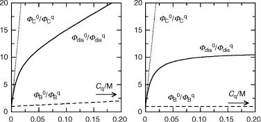
An example of the three Stern–Volmer functions is shown in Figure 3.26 (left). The parameters were assumed to be 1KSV ¼ 5 M 1, 3KSV ¼ 1000 M 1 and a ¼ FC0=FB0 ¼ 10. Even when the quenching constants 1kq and 3kq are the same, 3KSV is usually much larger than 1KSV, because the triplet lifetime is much longer. In the Figure 3.26 (right), 1KSV was set at zero, that is, we assumed that quenching of the singlet state is negligible, 1KSV 1. In that case, Equation 3.42 reduces to Equation 3.43. This is a common situation because singlet state lifetimes may be very short and because the singlet energy of the quencher is often higher than that of the quenchee, that is, 1kq 3kq. Alternant hydrocarbons have large singlet–triplet energy gaps, in contrast to triplet ketones (see Section 4.7). Thus, piperylene
Figure 3.26 Stern–Volmer diagrams for a two-step process (Scheme 3.3). Left: both S1 and T1 are quenched. Right: only triplet quenching is effective