

Photochemistry_of_Organic
.pdfEnergy Transfer, Quenching and Sensitization |
45 |
undergo many collisions, because the surrounding solvent molecules hinder their separation (FranckÐRabinowitch cage effect, Special Topic 6.11).
Reactions between molecules A and B via an encounter complex A B may be treated by the kinetic Scheme 2.3, where kd is equal to the bimolecular rate constant of diffusion, k d is the Þrst-order rate constant for escape from the encounter complex and kP is the Þrst-order rate constant of product formation in the encounter complex.
Scheme 2.3
The net rate of change of the encounter complex concentration cA B is equal to its rate of formation minus its rate of decay (Equation 2.25).
dcA B=dt ¼ kdcAcB ðk d þ kPÞcA B
Equation 2.25
The concentration cA B will be small compared with cA and cB throughout the reaction and after a short induction period its rate of formation will be largely balanced by its rate of decay, that is, we may assume dcA B/dt 0 (steady-state approximation). Rearrangement yields cA B kdcAcB/(k d þ kP) and the rate of product formation, dcP/dt ¼ kPcA B, is given by Equation 2.26.
kP dcP=dt kdcAcB k d þ kP
Equation 2.26
The partition ratio kP/(k d þ kP) deÞnes the efficiency of product formation from the encounter complex (see also Section 3.7.4). For the limiting case k d kP, where most encounters will be reactive, Equation 2.26 reduces to dcP/dt kdcAcB, that is, the overall observed rate constant of reaction approaches the rate constant of diffusion, kr kd. In 1917, von Smoluchowski derived Equation 2.27 from Fick s Þrst law of diffusion for the ideal case of large spherical solutes.
kd ¼ 4pr DNA
Equation 2.27 von Smoluchowski equation
The parameter r is the distance at which reaction occurs and of the diffusion coefÞcients of A and B. The latter can StokesÐEinstein Equation 2.28:
DA ¼ kBT
6phrA
D ¼ DA þ DB is the sum be calculated from the
Equation 2.28 Stokes–Einstein equation
where kB is the Boltzmann constant, h is the solvent viscosity, which is usually quoted in the non-SI unit poise (1 P ¼ 0.1 kg m 1 s 1 ¼ 0.1 Pa s), and rA is the radius of molecule A, which is assumed to be spherical and much larger than the solvent molecules. The SI units of diffusion coefÞcients are [D] ¼ m2 s 1.

46 |
Photophysics and Classification of Primary Photoreactions |
Having adopted various approximations up to this point, we may also assume that rA rB r /2 which, upon replacement of kBNA by the gas constant R, leads to Equation 2.29.
8RT kd ¼ 3h
Equation 2.29 Rate constant of diffusion of large spherical solutes
Note that r and the diffusion coefÞcient D have cancelled from Equation 2.29, because D is inversely proportional to the molecular radii r /2. Hence the rate constant kd depends only on temperature and solvent viscosity in this approximation. A selection of viscosities of common solvents and rate constants of diffusion as calculated by Equation 2.29 is given in Table 8.3. The effect of diffusion on bimolecular reaction rates is often studied by changing either the temperature or the solvent composition at a given temperature. For many solvents,54Ð56 although not for alcohols,57 the dependence of viscosity on temperature obeys an Arrhenius equation, that is, plots of log h versus 1/T are linear over a considerable range of temperatures and so are plots of log(kdh/T) versus 1/T.56
For solute molecules that are comparable in size to the solvent molecules or even smaller, Equation 2.29 yields values for kd that are too low, because small molecules can ÔslipÕ between the larger solvent molecules (see Section 2.2.5 on dioxygen). For small molecules, the von Smoluchowski Equation 2.27 gives more accurate predictions than the simpliÞed Equation 2.29, provided that diffusion coefÞcients and reaction distances r can be determined independently.58
The lifetime of encounter complexes between neutral reactants is on the order of 0.1 ns in solvents of low viscosity, that is, k d kd M. Random diffusive displacements of the order of a molecular diameter occur with a frequency of about 1011 s 1. Subsequently, the fragments from a speciÞc dissociation may re-encounter each other and undergo Ôsecondary recombinationÕ.59 If secondary recombination does not take place within about 1 ns, the fragments will almost certainly have diffused so far apart that the chance of a reencounter becomes negligible. The initial overall electronic multiplicity 2S þ 1 of encounter complexes is thus important in determining the fate of the reactants, because their lifetime is usually insufÞcient to allow for intersystem crossing during an encounter.
When the multiplicity of at least one of the reactants exceeds unity, we expand Scheme 2.3 to include the multiplicities m and n of the reactants (Scheme 2.4).53
Scheme 2.4
The product mn ¼ (2SA þ 1)(2SB þ 1) is the number of possible total spin angular momentum quantum numbers S of the encounter complex that are allowed by combination of the quantum numbers SA and SB of the reaction partners as deÞned by Equation 2.30.
S ¼ SA þ SB; SA þ SB 1; . . . ; jSA SBj
Equation 2.30
Energy Transfer, Quenching and Sensitization |
47 |
Because the energy differences dE between the sublevel states of each multiplet of mA and nB are very small, dE kT at ambient temperature and above, they are nearly equally populated under equilibrium conditions (Boltzmann s law, Equation 2.9) and the probability of the formation of any given encounter spin state will be equal to all the
others; as there are mn choices, it will be equal to the spin-statistical |
factor |
s ¼ ( |
mn) 1 |
. |
|||||||||
|
|
|
1 |
|
|
||||||||
For |
example, the multiplicity of radicals with one unpaired electron, S ¼ |
|
/2, |
is |
|||||||||
2S þ |
1 ¼ 2. Each of four |
spin states is then expected to form with equal probability upon |
|||||||||||
2 |
|
2 |
B, s ¼ 1/4. Three of these are sublevels of the encounter |
||||||||||
encounter of two radicals |
|
A and |
|
||||||||||
complex with triplet multiplicity, S ¼ SA þ SB ¼ 1, 2S þ 1 ¼ 3, and the |
fourth |
|
is |
the |
|||||||||
singlet encounter pair, S ¼ SA þ SB 1 ¼ 0, 2S þ 1 ¼ 1. Only the latter |
|
can undergo |
|||||||||||
radical recombination to form a singlet product P ¼AÐB without undergoing ISC. The above considerations therefore suggest that the rate constant for radical recombination will not exceed one-quarter of the rate constant of diffusion, because only every fourth encounter will lead to recombination.
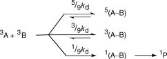
When two molecules in a triplet state collide, the spin quantum numbers SA ¼ SB ¼ 1 can combine to give the total spin quantum numbers S ¼ 2, 1 or 0 and the corresponding multiplicities of the encounter complex are 2S þ 1 ¼ 5, 3 or 1. If the only possible product P has singlet multiplicity, the statistical factor s for reaction is 1/9 (Scheme 2.5). Thus, observed rate constants for the quenching of triplet states by dioxygen producing singlet oxygen (Section 2.2.5) are generally no more than one-ninth of the diffusional rate constant for oxygen.60,61 Similarly, the formation of an excited singlet state by tripletÐtriplet annihilation (Equation 2.51) and the formation of the anthracene dimer62 (Scheme 6.90) upon encounter of two anthracene triplets are subject to a spin statistical factor of 1/9th.
Scheme 2.5
2.2.2Energy Transfer
Recommended textbooks.63,64
This section deals with processes by which the excitation energy of an excited molecule D , the energy donor, is transferred to a neighbouring molecule A, the energy acceptor (Equation 2.31). The multiplicity of D and A will be speciÞed as we look at the different mechanisms of energy transfer.
D* þ A ! D þ A*
Equation 2.31 Energy transfer
Energy transfer permits electronic excitation of molecules A that do not absorb the incident light. This is exploited, for example, for light harvesting in photosynthetic
48 |
Photophysics and Classification of Primary Photoreactions |
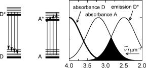
organisms. The energy absorbed by the antenna, which may consist of tens or even hundreds of chlorophyll molecules, is transported to the reactive centre, which then transforms it into storable chemical energy (Special Topics 6.25 and 6.26).65 We will consider only the lowest excited singlet and triplet state of the donor D because, under most conditions, internal conversion and vibrational relaxation (Section 2.1.1) from higher excited states of D will be much faster than any competing intermolecular energy transfer processes. Exceptions may occur in gases at very low pressure, where thermal relaxation is slow or when energy transfer is very rapid in systems containing high local concentrations of A.66 Energy transfer processes are isoenergetic: the energy lost by the donor reappears in the acceptor. If the electronic excitation energy of A is below that of D, an excited vibrational level of A will be populated initially and the excess energy is then rapidly dissipated to the medium rendering energy transfer irreversible (Figure 2.12, left).
Figure 2.12 Resonance condition for energy transfer from D to A. The thick horizontal bars in the left-hand diagram represent electronic and the thin bars vibrational states. The dark area on the right represents the spectral overlap integral J
Radiative energy transfer proceeds by way of electromagnetic radiation: a photon is spontaneously emitted by the excited donor D and subsequently absorbed by the acceptor A. This is by far the dominant process of energy transport in dilute gases as in interstellar space. Radiative energy transfer was considered in the derivation of Planck s law for the frequency distribution of a black-body radiator (Special Topic 2.1). It is sometimes referred to as trivial energy transfer, because it is conceptually simple and must be taken into account under any circumstances. However, we shall see that it is usually not the dominant energy transfer process, except in very large, dilute systems, where intermolecular interactions are negligible. The absorption spectrum of A must overlap with the emission spectrum of D for A to absorb a photon emitted by D (Figure 2.12, right).
The probability p that a photon emitted by D will be absorbed by A is given by Equation 2.32:
p ¼ ð In~D*½1 10 Aðn~Þ& dn~ |
|
where In~D* ¼ In~D*n~ ð In~D*dn~; that is |
ð In~D*dn~ ¼ 1 |
n~ |
n~ |
Equation 2.32 Probability of radiative energy transfer from D to A

Energy Transfer, Quenching and Sensitization |
49 |
|||
where the normalized spectral radiant intensity |
m,10,22 |
D* |
represents |
the spectral |
|
In~ |
|||
distribution of the ßuorescence emission by D and the term 10 Aðn~Þ is equal to the transmittance T(n~) from the point of emission by D to the bounds of the solution. Equation 2.32 is readily derived by considering the probability for reabsorption of a
|
D* |
½1 Tðn~Þ&dn~. |
|
I |
|
photon in a given wavenumber interval dn~, dp ¼A n~ |
||
Taylor expansion of the exponential term, 10 |
1 Ð ln(10)A, neglecting higher terms |
|
and replacement of A(n~) by «A(n~)cA‘ gives the approximate expression Equation 2.33, which holds for low absorbances A. The probability p for energy transfer is then proportional to the concentration cA, to the average optical pathlength ‘ of emitted photons travelling through the solution that depends on the size and the shape of the sample and to the spectral overlap integral J (Figure 2.12). The spectral distributions of the emission by
D* ~
D , In~ , and of the absorption by A, «A(n), are normalized by deÞnition, so that the overlap integrals Jn ¼ Jl do not depend on the oscillator strengths of the transitions involved.
|
p 2:303cA‘J |
|
|
where Jn~ |
¼ ð In~D*«Aðn~Þdn~; |
ð In~D*dn~ ð «Aðn~Þdn~ 1 |
|
|
n~ |
n~ |
n~ |
and |
Jl ¼ ð IlD*«AðlÞdl; |
ð IlD*dl |
ð «AðlÞdl 1 |
|
l |
l |
l |
Equation 2.33 Probability of radiative energy transfer from D to A
Radiative energy transfer between identical molecules tends to increase the apparent lifetime of the emitting species D because photons already emitted are being recaptured. However, it rarely occurs, because the overlap integral J is necessarily small for D ¼A (Figure 2.12). For D 6¼A, on the other hand, J may approach unity in favourable cases. Yet radiative energy transfer from D to acceptors A does not affect the lifetime of D ; it occurs only when D emits spontaneously and it is irreversible when the excitation energy of A is lower than that of D due to the rapid dissipation of excess vibrational energy on A .
In practice, it is usually observed that the ßuorescence lifetime (Section 3.5) and quantum yield (Section 2.1.7) of D decrease when an acceptor A is added, a phenomenon called concentration quenching. Clearly, some interactions between D and A play a role. Energy transfer processes that reduce the lifetime of D cannot be attributed to the spontaneous emission of a photon by D and are thus called nonradiative energy transfer processes (stimulated energy transfer would also be an appropriate expression, but is rarely used). Moreover, Pringsheim noted in 1924 that the polarization of ßuorescence (Section 3.6) decreases rapidly with increasing concentration of D in solid solutions, much more so than could reasonably be explained on the basis of radiative energy transfer that, moreover, should have depended on the sample size, but did not. In the same year, Perrin attributed ßuorescence depolarization to nonradiative energy transfer and offered a classical electrodynamic model to explain energy transfer over large distances. Perrin later provided
m Radiant intensity, I, is the radiant power (Equation 2.3), P, per solid angle, V, emitted at1 all wavelengths, I ¼ dP/dV. If the |
|||||||||||||||||
radiant power is constant over the solid angle considered, I ¼ P/V. The unit of I is W sr |
. The spectral radiant intensity is |
||||||||||||||||
the |
derivative |
of |
radiant |
intensity |
with respect to wavelength or wavenumber, I |
l ¼ |
dI/d |
l |
, |
|
dI/dv. The SI units are |
||||||
I |
|||||||||||||||||
|
|
1 |
|
1 |
|
|
|
1 |
|
|
|
|
~v ¼ |
~ |
|||
[Il] ¼ W m |
|
sr |
|
|
|
. |
|
|
|
|
|
|
|
||||
|
|
|
and I~v ¼ W m sr |
|
|
|
|
|
|
|
|
|
|||||

50 |
Photophysics and Classification of Primary Photoreactions |
a quantum mechanical interpretation, but neither model could reproduce the available data accurately.
The analogy to a radio emitter and receiver is sometimes used to visualize energy transfer. This analogy is adequate for radiative but not for nonradiative energy transfer, because in the latter process the emitter is stimulated by the acceptor to forsake its excitation energy.
A quantum mechanical treatment of nonradiative energy transfer is based on Fermi s
¼ hC j^jC i
golden rule (Equation 2.21). The interaction term Vif i h f , which couples the (initial) zero-order wavefunction Ci ¼ CD CA of the neighbouring molecules prior to energy transfer with the wavefunction Cf ¼ CDCA of the Þnal state, permits energy transfer over extended distances without the intervention of a photon. The Coulombic
interactions contained in the perturbation operator ^ may be expanded as a multipole h
series. If the intermolecular distances are much larger than the size of the molecules, the Þrst term, representing the dipoleÐdipole interaction between the transition moments of the donor D and of the acceptor A, predominates for allowed transitions. As the interaction between two point-dipoles falls off with the third power of the distance, the rate constant for F€orster-type resonance energy transfer (FRET),n kFRET, being proportional to Vif2 (Equation 2.21), falls off with the sixth power of the distance R between D and A (Equation 2.34):
kFRET ¼ R60=ðR6t0DÞ
Equation 2.34 Forster€ resonance energy transfer
where t0D is the lifetime of D in the absence of acceptor molecules A and R0 is called the critical transfer distance. When the distance R equals R0, kFRET ¼ 1=t0D, energy transfer and spontaneous decay have equal rate constants and these processes are equally probable. Note that the rate constant kFRET is a Þrst-order rate constant, [kFRET] ¼ s 1. It pertains to the rate of energy transfer between D and A that are being held at Þxed distance and relative orientation.
By applying Fermi s golden rule, F€orster derived a very important relation between the
critical transfer distance R0 and experimentally accessible spectral quantities (Equation 2.35),o, 67,68 namely the luminescence quantum yield of the donor in the absence of
acceptor A, F0D, the orientation factor, k, the average refractive index of the medium in the region of spectral overlap, n, and the spectral overlap integral, J. The quantities J and k will be deÞned below. Equation 2.35 yields remarkably consistent values for the distance between donor and acceptor chromophores D and A, when this distance is known. FRET is, therefore, widely applied to determine the distance between markers D and A that are attached to biopolymers, for example, whose tertiary structure is not known and thus
nThe term FRET was Þrst used in papers relevant to life sciences as an acronym for Ôßuorescence resonance energy transferÕ. This is a misnomer, because ßuorescence is not involved in the transfer, which is nonradiative. The term RET (resonance energy transfer) would be more appropriate, but it is also used for Ôreturn electron transferÕ (Section 5.4.3). Because FRET is an established acronym, the letter ÔFÕ is now taken to stand for ÔF€orster, or F€orster-typeÕ.
oÔFor F€orster s scholars in Stuttgart this book was so to speak the house bible, a quite appropriate designation, for one because it provided the means of understanding and second because of its precise and concise style, where each word mattered and many sentences required very careful reading and re-reading or Ð better still Ð the exegesis by an interpreter, before one could grasp its superb content. For those not conversant in German it must have largely remained a book with seven seals; because it was not translated into English, American colleagues say that it secured a German lead in ßuorescence spectroscopy for years.Õ [Translated from the obituary of F€orster given by Albert Weller, 1974].

Energy Transfer, Quenching and Sensitization |
51 |
serves as a Òmolecular rulerÕÕ (Special Topic 2.3).
R6 |
¼ |
9lnð10Þ |
|
k2FD0 |
J |
0 |
128p5NA |
|
n4 |
|
Equation 2.35 Forster€ s equation to calculate the critical transfer distance R0 was erroneously printed with p6 instead of p5 in the denominator in several papers by Forster€ . He corrected this misprint in a later publication.69,70,p
The spectral overlap integral J can be expressed in terms of either wavenumbers or wavelengths (Equation 2.36). The area covered by the emission spectrum of D is
D* |
D* |
are the normalized spectral radiant |
normalized by deÞnition and the quantities In~ |
and Il |
intensities of the donor D expressed in wavenumbers and wavelengths, respectively. Note that the spectral overlap integrals J deÞned here differ from those relevant for radiative energy transfer (Equation 2.33). Only the spectral distributions of the emission by D ,
D* |
D* |
, are normalized, whereas the transition moment for excitation of A enters |
In~ |
and Il |
|
explicitly by way of the molar absorption coefÞcient «A. The integrals Jn~ and Jl are equal, |
||
because the emission spectrum of D is normalized to unit area and the absorption
coefÞcients «A are equal on both scales. |
; |
Jl ¼ |
ð Il «AðlÞl4dl; |
|||
|
Jn~ ¼ ð In~D*«Aðn~Þ n~4 |
|||||
|
|
|
dn~ |
|
D* |
|
|
n~ |
|
|
|
ð |
l |
|
ð |
|
|
|
|
|
where |
D* |
dn~ 1 and |
D* |
dl 1 |
||
In~ |
Il |
|||||
|
n~ |
|
|
|
l |
|
Equation 2.36 Spectral overlap integral for nonradiative energy transfer
Collecting the numerical constants and length conversion factors, we obtain the practical expression Equation 2.37. The proportionality constant will differ for a different choice of units. It is unnecessary and not recommended to convert the emission spectrum of the donor to a wavenumber scale for the calculation of J (see Section 3.4).
|
|
|
|
|
|
k2F0 |
|
Jl |
|
1 |
|
R0 |
¼ 0:02108 |
|
|
6 |
|||||
|
|
|
D |
|
|
|
||||
|
nm |
n4 |
mol 1 dm3 cm 1 nm4 |
|
||||||
|
|
|
Equation 2.37 Practical expression for R0 |
|
||||||
The variables n~ and l in J |
n~ |
l |
|
|
|
|
|
|||
|
and J are sometimes replaced by constant average values n~ |
|||||||||
and , respectively, representing the positions of maximum spectral overlap, so that they can l
be moved in front of the integrals J. The orientation factor k is deÞned by Equation 2.38:
k ¼ mDmA 3ðmDrÞðmArÞ mDmA
Equation 2.38 Orientation factor
p In Equation 2.3, the units can be chosen arbitrarily, as long as their product is the same on both sides. Most papers, reviews and textbooks show a factor of 9000 rather than 9 in the numerator. Apparently, this is done to convert dm3 (appearing in the molar absorption coefÞcient «) to cm3. Equation 2.35 with a factor of 9000 no longer has equal units on both sides (caveat emptor!). Such confusing and unnecessary practice should be avoided. When doing such a conversion, the units must be given explicitly, as in the scaled Equation 2.37.70
52 |
Photophysics and Classification of Primary Photoreactions |
Figure 2.13 Angles defining the orientation factor k
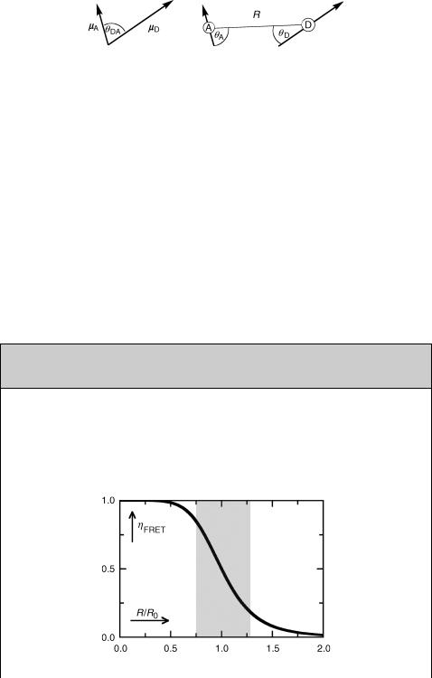
where mD and mA are the transition moment vectors of D and A and r is the unit vector in the direction of R. Possible values for k2 range from 0 to 4 depending on the relative orientation of the transition dipole moments mD and mA. The relevant angles are deÞned in Figure 2.13; k2 ¼ 0 when the electric Þeld generated by mD is perpendicular to mA, that is, when uDA ¼ uD ¼ 90 or uDA ¼ uA ¼ 90 or when the two terms in the numerator of Equation 2.38 cancel; k2 ¼ 4 when all vectors are in line, uDA ¼ uD ¼ uA ¼ 0 .
Two issues require careful consideration. The Þrst is the effect of diffusion on energy transfer rates in media of low viscosity, which will be considered below. The second is the choice of an appropriate orientation factor k. For FRET in solution, it is usually warranted to assume that the molecules D and A undergo rapid Brownian rotation during the lifetime of D . Averaging over all possible orientations of the transition dipoles gives hk2i ¼ 2/3. If the dipoles are randomly oriented but do not rotate on the time scale of the donor luminescence in rigid media, other average values must be used, for example h|k|i2 ¼ 0.476 for large three-dimensional samples.71 Concerns72 that the use of hk2i ¼ 2/3 may be inadequate, when ßuorescent labels are attached to speciÞc sites of biopolymers such as enzymes or DNA in order to determine the distance between these sites from observed FRET efÞciencies, have been dispelled.73
Special Topic 2.3: Energy transfer – a tool to measure distances and to track the motion of biopolymers
The efÞciency (Equation 3.32, Section 3.9.7) of FRET is deÞned as hFRET ¼ kFRET/ (kFRET þ 1/t0D). Inserting Equation 2.34 for kFRET one obtains Equation 2.39. This function falls off rapidly as R exceeds the critical F€orster radius R0, Figure 2.14.
hFRET ¼ R60=ðR60 þ R6Þ
Equation 2.39 Efficiency hFRET as a function of distance
Figure 2.14 Efficiency hFRET as a function of distance

Energy Transfer, Quenching and Sensitization |
53 |
Having attached a donor chromophore D and an acceptor A to speciÞc sites of a biopolymer such as a DNA hairpin or an enzyme, the efÞciency of FRET is measured by comparing the steady-state ßuorescence signal intensity of the donor D in the presence and absence of the acceptor A under otherwise identical conditions, hFRET ¼ 1 Ð Il0/IlA. The critical F€orster radius R0 is calculated from the spectral properties of D and A (Equation 2.37). With the experimental for value hFRET, Equation 2.39
deÞnes the apparent donorÐacceptor distance, R |
¼ |
Rapp (Equation 2.40); hence the |
||
|
|
|
74,75 |
|
expressions Ômolecular rulerÕ or Ôspectroscopic rulerÕ. |
||||
IA |
1=6 |
|
||
|
|
|
||
Rapp ¼ R0 Il0 |
|
|
||
|
l |
|
|
|
Equation 2.40 FRET as a molecular ruler
When the distance R between D and A can be calculated or measured by other methods in relatively rigid systems, it has been amply demonstrated that remarkably consistent values of Rapp are obtained from FRET measurements. However, Rapp may differ somewhat from the actual donorÐacceptor distance in a ßexible macromolecule with a broad distribution of donorÐacceptor distances. The distance Rapp derived from steady-state FRET measurements then considerably overestimates the true mean distance.76 To treat ßexible macromolecules or conformational mixtures, time-resolved measurements of FRET are necessary.75
In recent years, single-molecule spectroscopy (SMS) (Section 3.13) has been successfully applied to probe the free-energy surfaces that govern protein folding.77 Moving away from ensemble measurements is an essential step forward in applications of FRET.78Ð82 The conformational changes undergone by a single, denatured protein molecule in search of its native structure are recorded in a ÔdiaryÕ as FRET is repeatedly switched off and on (Figure 2.15). Ideally, one would like to record the dynamics on the reconÞguration time scale of single polypeptide chains as they wiggle their way through the energy landscape, each molecule taking its own route to the folded state. Similarly, single-molecule FRET can visualize enzymes at work by monitoring conformational changes during substrate conversion.83 SMS using FRET will continue to attract widespread attention.
Figure 2.15 The empty circles represent the ground state and filled circles the excited state of D or A

54 |
Photophysics and Classification of Primary Photoreactions |
In 1969, Levinthal posed his famous paradox pointing out that the conÞgurational space of a polypeptide chain is so large that it can never Þnd its native conformation by a random search. Evolution has apparently selected polypeptide chains that Þnd their native fold reliably and quickly. Their free-energy landscapes exhibit minimal ruggedness and the overall shape of a funnel with only shallow local minima.
Rate constants ket for tripletÐtriplet energy transfer (TET) in ßexible bichromophoric systems DÐ(CH2)nÐA were determined from steady-state quenching and quantum yield measurements. The magnitude of ket for n ¼ 3 is comparable to that in molecules with a rigid spacer between the chromophores, so that a through-bond mechanism is assumed to remain important. As the connecting polymethylene chain becomes longer, a gradual drop in TET rate constants indicates that through-space interactions, that is, encounter contacts between 3D and A, enabled by rapid conformational equilibria, compete and provide the only mechanism responsible for transfer when n 5.84,85
The elementary steps of peptide folding are single-bond conformational changes, which occur on a picosecond time scale. Intrachain loop formation allows unfolded polypeptide chains to search for favourable interactions during protein folding. The dynamics on the nanosecond time scale represent chain diffusion exploring different local minima on the free energy landscape. TripletÐtriplet energy transfer is thus ideally suited to monitor rates of contact formation in polypeptide chains and to explore the early dynamics of peptide folding.86Ð88 As an alternative, the long-lived ßuorescent state of 2,3-diazabicyclo[2.2.2]oct-2-ene (DBO) was used to monitor contact quenching in oligopeptide chains giving largely consistent results.89,90 The kinetics of end-to-end collision in single-stranded oligodeoxyribonucleotides of the type 50- DBOÐ(X)nÐdG (X ¼ dA, dC, dT or dU and n ¼ 2 or 4) was investigated by the same method. The ßuorophore was covalently attached to the 50 end and dG was introduced as an efÞcient intrinsic quencher at the 30 terminus.91
Conditions of FRET from singlet donors 1D* to acceptors A in the singlet ground state are optimal when the excitation energy of the acceptor is somewhat lower than that of the donor, ensuring good spectral overlap. FRET between identical molecules, D ¼A, is relatively slow, especially at low temperatures, where overlap is restricted to the 0Ð0 transition. At higher temperatures, the overlap increases somewhat due to thermal population of some excited vibrational levels of 1D*. In single crystals, repeated energy transfer can proceed over large distances until the excitation arrives at an impurity trap of lower energy. Fascinating studies of FRET between chromophores in organized systems such as zeolites loaded with chromophores,92 monolayer assemblies93 and self-assembling
columnar mesophases,94Ð96 in dendrimers97,98 and in other covalently linked chromophores that can be used as molecular switches, multiplexers99,100 or antenna molecules,101,102 have been reported. In such closely associated systems of m donor and
n acceptor chromophores, simple models considering only pairwise interactions between nearest neighbours may be inadequate. Rather, all m n electronic couplings should be considered simultaneously, which leads to a more delocalized model and even faster rates of energy transfer (exciton hopping).103
Equation 2.37 predicts very short transfer distances R0 for forbidden transitions of A, such as in singletÐtriplet transfer to organic acceptor molecules that have very low