

Photochemistry_of_Organic
.pdf4 |
Introduction |
Figure 1.2 Left: human energy consumption rate. Current per capita rate 2300 W (EU 6000 W, USA 12 000 W). Right: night-time satellite picture of Africa and Europe showing the distribution of artificial light sources
off, as shown in Figure 1.2 (left) (notwithstanding the developing nations’ expected growing energy demand; Figure 1.2, right), it is far from clear how the gap will be filled when the sources of fossil fuels are exhausted, and whether the demand that their consumption be strongly curtailed to reduce the rate of global warming can be met. Uranium ores worth exploiting are also limited, leaving few conceivable options for substantial contributions through sustainable technology, primarily solar energy storage (photovoltaics, hydrogen production), nuclear fusion, wind energy, sea tide and geothermal sources. Major efforts to increase the efficiency of all processes requiring energy and to find substitutes for energy-demanding behaviour will be needed to balance the worldwide energy demand against our non-renewable resources during this century. Light-driven processes will be a major contributor in the transformation to a low-carbon economy.7 The production of photovoltaic cells is currently rising at a pace of about 40% per year. More dramatic increases in the exploitation of renewable energy sources will follow as soon as these techniques can compete with the rising cost of fossil fuels.
A remarkably detailed understanding of the properties and chemical behaviour of transient intermediates has been deduced from well-designed conventional methods of physical organic chemistry using standard laboratory techniques such as quenching and sensitization, trapping or radical clocks. However, working backwards from the structure of stable photoproducts and the variation of their yield as a function of various additives requires demanding preparative and analytical efforts; moreover, the lifetimes of intermediates can only be estimated from such data by making some assumptions about the rate constants of quenching or trapping (Section 3.9.6). On the other hand, flash photolysis (Section 3.7) provides absolute rate constants with little effort, but yields precious little hard information allowing the identification of the observed transients. Kinetic data obtained by optical flash photolysis alone are thus prone to false assignments and the combination of both methods is highly recommended. Once a hypothetical reaction mechanism has been advanced, the quantitative comparison of

Who’s Afraid of Photochemistry |
5 |
the effect of added reagents on product distributions, quantum yields and transient kinetics provides a stringent test for the assignment of the transients observed by flash photolysis (Section 3.9.8, Equation 3.38). Other time-resolved spectroscopic techniques such as MS, IR, Raman, EPR, CIDNP and X-ray diffraction provide detailed structural information permitting unambiguous assignment of transient intermediates and their chemical and physical properties can now be determined under most conditions.
Special Topic 1.1: Historical remarks
Many of the above considerations regarding the impact of photochemistry on the future of mankind were expressed 100 years ago in prophetic statements by Giacomo Luigi Ciamician (1857–1922).8,9 The first attempts to relate the colour of organic compounds to their molecular structure date back to the mid-19th century, when synthetic dyes became one of the chemical industry’s most important products. In 1876, Witt introduced the terms chromophore (a molecular group that carries the potential for generating colour) and auxochrome (polar substituents that increase the depth of colour). Dilthey, Witzinger and others further developed the basic model. Such colour theories had to remain empirical and rather mystical until the advent of molecular quantum mechanics after 1930, and it took another 20 years until simple molecular orbital theories such as Platt’s free electron model (FEMO), H€uckel molecular orbital theory (HMO) and Pariser, Parr and Pople’s configuration interaction model (PPP SCF CI) provided lucid and satisfactory models for the interpretation of electronic spectra of conjugated molecules. Such models were also successful in rationalizing trends in series of related molecules and in describing the electronic structure and reactivity of excited states.
More sophisticated ab initio methods can and will increasingly provide accurate predictions of excited-state energies, transition moments and excited-state potential energy surfaces of fairly large organic molecules. However, these methods are less amenable to generalization, intuitive insight or prediction of substituent effects. The translation of quantitative ab initio results into the language of simple and lucid MO theories will remain a necessity.
General lines of thought on how to understand the reactivity of electronically excited molecules emerged only after 1950. T. Fo¨rster, M. Kasha, G. Porter, E. Havinga, G. Hammond, H. Zimmerman, J. Michl, N. Turro and L. Salem were among the intellectual leaders who developed the basic concepts for structure– reactivity correlations in photochemistry (Section 4.1). Spectroscopic techniques together with computational methods began to provide adequate characterization of excited states and their electronic structure. Simple models such as correlation diagrams were used for the qualitative prediction of potential energy surfaces. Matrix isolation at cryogenic temperatures permitted the unambiguous identification of reactive intermediates.
The rapid development of commercially available lasers and electronic equipment allowed for the real-time detection of primary transient intermediates by flash photolysis. Photochemistry thus emerged as the principal science for the study of
6 |
Introduction |
organic reaction mechanisms in general, because it can be employed to generate the intermediates that are postulated to intervene in chemical reactions of the ground state. Cutting edge research provides unprecedented spatial and temporal resolution to monitor structural dynamics with atomic-scale resolution, to detect single enzyme or DNA molecules at work and to construct light-driven molecular devices.
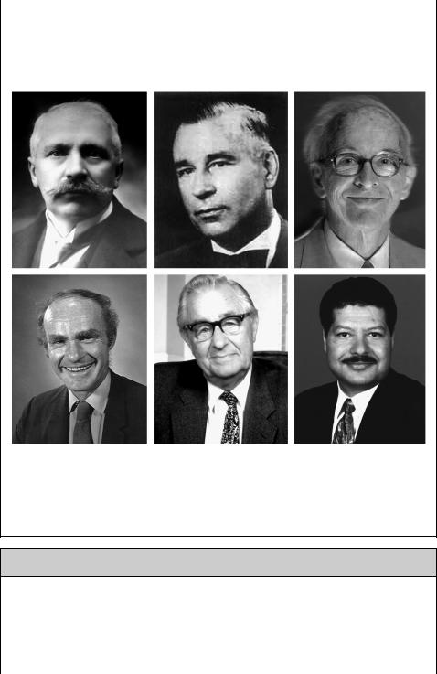
Figure 1.3 Some of photochemistry’s icons. Top (from left to right): Giacomo Ciamician (1857–1922), Theodor Fo¨rster (1910–1974), Michael Kasha (1920–). Bottom: George Hammond (1921–2005), George Porter (1920–2002), Ahmed Zewail (1946–). Photographs reproduced by permission of the Scientists (M. K., A. Z.), or of successors at their former institutions
Special Topic 1.2: Quantity calculus
By convention, physical quantities are organized in the International System (SI) of quantities and units, which is built upon seven base quantities (Table 1.1), each of which is regarded as having its own dimension. The current definitions of the corresponding base units are given in the IUPAC Green Book, Quantities, Units and Symbols in Physical Chemistry.10 A clear distinction should be drawn between the names of units and their symbols, e.g. mole and mol, respectively.

Who’s Afraid of Photochemistry |
|
|
7 |
||||
Table 1.1 The SI base quantities |
|
|
|
|
|
|
|
|
|
|
|
|
|
|
|
Base quantity |
|
|
SI unit |
|
|
|
|
|
|
|
|
|
|
|
|
Name |
Symbol for |
Symbol for |
|
Name |
Symbol |
||
|
quantity |
dimension |
|
|
|
|
|
|
|
|
|
|
|
||
Length |
l |
L |
metre |
m |
|||
Mass |
m |
M |
kilogram |
kg |
|||
Time |
t |
T |
|
second |
s |
||
Electric current |
I |
I |
|
ampere |
A |
||
Thermodynamic temperature |
T |
Q |
|
kelvin |
K |
||
Amount of substance |
n |
N |
|
mole |
mol |
||
Luminous intensity |
IV |
J |
|
candela |
cd |
|
|
A measurement amounts to the comparison of an object with a reference quantity of the same dimension (e.g. by holding a metre stick to an object). The value of a physical quantity Q can be expressed as the product of a numerical value or measure, {Q}, and the associated unit [Q], Equation 1.1.
Q ¼ fQg½Q&; e:g:; h ¼ 6:626 10 34 J s
Equation 1.1
The symbols used to denote units are printed in roman font; those denoting physical quantities or mathematical variables are printed in italics and should generally be single letters that may be further specified by subscripts and superscripts, if required. The unit of any physical quantity can be expressed as a product of the SI base units, the exponents of which are integer numbers, e.g. [E] ¼ m2 kg s 2. Dimensionless physical quantities, more properly called quantities of dimension one, are purely numerical physical quantities such as the refractive index n of a solvent. A physical quantity being the product of a number and a unit, the unit of a dimensionless quantity is also one, because the neutral element of multiplication is one, not zero.
Quantity calculus, the manipulation of numerical values, physical quantities and units, obeys the ordinary rules of algebra.11 Combined units are separated by a space, e.g. J K 1 mol 1. The ratio of a physical quantity and its unit, Q=½Q&, is a pure number. Functions of physical quantities must be expressed as functions of pure numbers, e.g. logðk=s 1Þ or sin(vt). The scaled quantities Q=½Q& are particularly useful for headings in tables and axis labels in graphs, where pure numbers appear in the table entries or on the axes of the graph. We will also make extensive use of scaled quantities Q=½Q& in practical engineering equations. Such equations are very convenient for repeated use and it is immediately clear, which units must be used in applying them. For example, a practical form of the ideal gas equation is shown in Equation 1.2.
p ¼ 8:3145 |
n T |
|
V |
|
1 |
||
|
|
|
|
Pa |
|||
mol |
K |
m3 |
|||||
Equation 1.2
8 |
Introduction |
If the pressure is required in psi units, the equation can be multiplied by the conversion factor 1.4504 10 4 psi/Pa ¼ 1 to give Equation 1.3.
|
n T |
|
V |
1 |
||||
p ¼ 1:206 10 3 |
|
|
|
|
|
|
|
psi |
mol |
K |
m3 |
||||||
Equation 1.3 |
|
|
|
|
||||
In this text, the symbols H þ and e generally used by chemists are adopted as |
||||||||
symbols for the proton and electron, rather than p and e, respectively, as recommended |
||||||||
by IUPAC. The symbol e represents the elementary charge; the charge of the electron is |
||||||||
–e, that of the proton is e. In chemical schemes these charges will be represented by |
||||||||
and , respectively. Some fundamental physical quantities and energy conversion |
||||||||
factors are given in Tables 8.1 and 8.2. |
|
|
|
|
||||
1.2 Electromagnetic Radiation
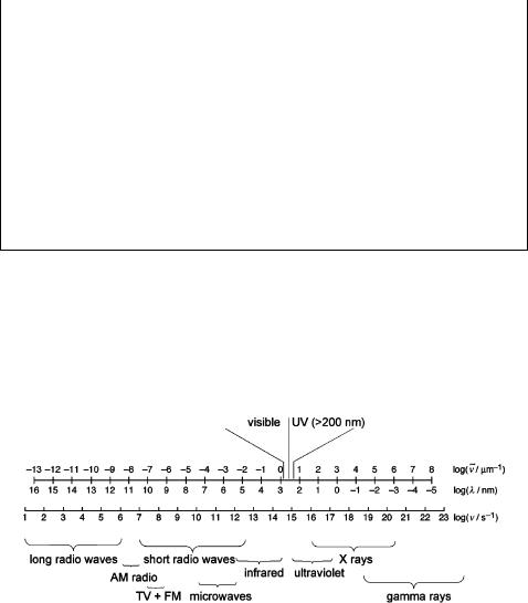
We are dealing with the interactions of light and matter. The expression light is used here somewhat loosely to include the near-ultraviolet (UV, l ¼ 200–400 nm) and visible regions (VIS, l ¼ 400–700 nm) of the entire electromagnetic spectrum (Figure 1.4), which spans over 20 orders of magnitude.
Figure 1.4 Electromagnetic spectrum
The first law of photochemistry (Grothus, 1817; Draper, 1843) states that only absorbed light is effective in photochemical transformation.
The second law of photochemistry (Einstein, 1905) states that light absorption is a quantum process. Usually, one photon is absorbed by a single molecule.
The particle nature of light was postulated in 1905 by Einstein to explain the photoelectric effect. When light is incident on a metal surface in an evacuated tube, electrons may be ejected from the metal. This is the operational basis of photomultipliers and image intensifiers, which transform light to an amplified electric signal (see Section 3.1).
Electromagnetic Radiation |
9 |
The kinetic energy of these electrons is independent of the light intensity. This surprising result was not understood until Einstein proposed that light energy is quantized in small packets called photons. The photon is the quantum of electromagnetic energy, the smallest possible amount of light at a given frequency n. A photon’s energy is given by the Einstein equation (Equation 1.4), where h ¼ 6.626 10 34 J s is Planck’s constant.b
Ep ¼ hn
Equation 1.4
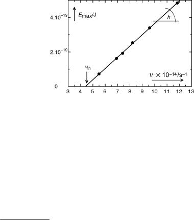
Einstein made the bold prediction that photons with an energy below that needed to remove an electron from a particular metal would not be able to eject an electron, so that light of a frequency below a certain threshold nth would not give rise to a photoelectric effect, no matter how high the light intensity. Moreover, he predicted that a plot of the photoelectrons’ maximum kinetic energy, Emax, against the frequency of light n should be a straight line with a slope of h (Figure 1.5). R. A. Millikan verified this 10 years later.12
Figure 1.5 Maximum kinetic photoelectron energy Emax ejected from sodium metal as a function of light frequency. Adapted from ref. 12
|
frequency n of light is inversely proportional to its wavelength |
l |
, n |
¼ |
c/ , where |
|||||||||||||
The |
|
8 |
m s |
1 |
is the speed |
of light; it is often replaced |
|
|
|
l |
|
|
||||||
c ¼ 2.998 10 |
|
|
|
by the wavenumber, |
||||||||||||||
n~ ¼ n=c ¼ 1=l, which corresponds to the number of waves per |
unit |
length. The |
SI |
|||||||||||||||
1 |
||||||||||||||||||
|
1 |
½ |
n |
& ¼ |
s 1 and |
½ |
n~ |
& ¼ |
|
1 |
|
|
|
|
|
1 |
|
|
base units are |
|
|
|
|
m 1. We will generally use the derived units cm |
|||||||||||||
(¼ 100 m ) for wavenumbers of vibrational transitions and mm |
|
(¼ 10 000 cm ) for |
||||||||||||||||
wavenumbers of electronic transitions. |
|
|
|
|
|
|
|
|
||||||||||
The energy transferred to a molecule by the absorption of a photon is DE |
¼ hn ¼ hcn~. |
|||||
The energy of 1 mol |
of photons (1 einstein), |
l |
300 nm, amounts |
to N |
AEp ¼ |
|
NAhcn~ 400 kJ mol |
1 |
|
|
|
||
|
and is sufficient for the homolytic cleavage of just about any single |
|||||
bond in organic molecules. For example, a similar amount of energy would be taken up by
b The constant h was introduced in 1899 by Max Planck to derive a formula reproducing the intensity distribution of a black-body radiator (Section 2.1.3). To this end, Planck had to assume that a hot body emits light in quanta of energy hn, but he considered this assumption to be an amazing mathematical trick rather than a fundamental property of nature.
10 |
Introduction |
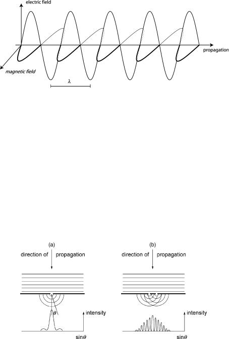
Figure 1.6 Electromagnetic wave along a propagation axis x. Note the scaling parameter l. For l ¼ 300 nm, a full wave spans a length that is more than two orders of magnitude larger than that of an average molecule. The propagation axis could be replaced by time t to indicate the electromagnetic wave’s oscillations at a given point in space. For a light wave of l ¼ 300 nm, the scale shown would then represent a time span of 10 15 s
naphthalene [Cp,m(g) ¼ 136 J K 1 mol 1] if it were immersed in a heat bath at 3000 K. This might suggest that organic molecules are indiscriminately destroyed by irradiation with UV light. Fortunately, this is not the case and we shall see why. The physical description of light is mind-boggling. Classical optics can be fully understood by mathematically treating light beams as electromagnetic waves (Figure 1.6).
Other phenomena are best described in terms of light’s particle nature (Equation 1.4). These seemingly contradictory properties are inseparable parts of the dual nature of light. Both must be taken into account when considering a simple process such as the absorption of light by matter. The above statements will surprise few readers because they have heard them many times before. But consider the experiment depicted in Figure 1.7.
Figure 1.7 Parallel waves (representing either light or water waves in a ripple tank) encountering a barrier with (a) one small slit producing diffraction and (b) two small slits whose separation is equal to 10 times their width, producing an interference–diffraction pattern

Perception of Colour |
11 |
The diffraction patterns generated by parallel waves encountering a barrier with (a) one or (b) two holes (Figure 1.7) are predicted by the wave theory of light. The peaks and troughs appearing in the intensity distribution of the right-hand diagram with two slits are due to constructive and destructive interference of the diffracted light beams emerging from the two slits. What happens when the distant light source’s intensity is reduced so much that only one photon arrives at the barrier per second? Now the photons cannot interact with each other while passing the barrier and they will be registered one at a time when they hit the detector screen. However, if we wait long enough to obtain good statistics on the intensity distribution, we will get exactly the same pattern of peaks and troughs as with a strong light source. Thus a single photon approaching barrier (b) in Figure 1.7 near the two holes has wave-like properties and will exhibit interference with itself’ while passing one of the barrier’s slits!c In Section 1.4, we shall see that electrons, which in classical physics can be treated as particles carrying the elementary charge e, e ¼ 1.602 10 19 C, also exhibit wave-like properties.
1.3 Perception of Colour
Recommended review.13
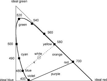
Vision is initiated by the absorption of light in the eye’s retina, which hosts about 5 million cone cells and 90 million rod cells (Special Topic 6.1). Humans have three kinds of cones with different response curves. The cones are less sensitive to light than the rods (which support vision at low light levels), but they allow the perception of colour. Moreover, their response times to stimuli are faster than those of rods. An attempt to chart colours in a triangle of three primary light sources goes back to Maxwell. The modified diagram shown in Figure 1.8 was defined in 1931 by the International Commission on Illumination. Pure spectral colours, those seen by looking at a monochromatic light source, are located on the curved solid line from violet (400 nm) to red (700 nm). The straight line connecting 380 and 700 nm at the bottom represents the non-spectral colours of purple that can be obtained by mixing violet and red light.
Any colour perceived by direct viewing of a light source corresponds to a point in the area enclosed by the curved line and the tilted bottom line. Following the dotted line in Figure 1.8, we would proceed from spectral (or saturated) blue (480 nm) through pale blue, white and pale yellow to saturated yellow (580 nm). A pair of colours that can produce the sensation of white’, i.e. which can be joined by a straight line that passes through the white point, is called a complementary pair. Thus blue and yellow form a complementary pair, as do orange (600 nm) and blue–green (488 nm), also called cyan’. Such colours are called additive colours. Physically, spectral yellow (580 nm) is clearly different from a mixture of red (700 nm) and green light (520 nm). However, both stimulate our eyes in a similar manner, so we do not notice that difference. The additive reproduction process usually uses red, green and blue light (RGB) to produce the other colours. Combining one of these additive primary colours with another in equal amounts produces the additive secondary colours cyan, magenta and yellow (CMYK, K for black). Combining all three
c I am afraid I can’t put it more clearly’, Alice replied very politely, for I can’t understand it myself to begin with’ (Lewis Carroll, Alice in Wonderland). We all know what light is, but it is difficult to tell what it is.’ (Samuel Johnson).
12 |
Introduction |
Figure 1.8 Colour triangle . Any perceived colour is represented by a point in the area enclosed by the curved line. The wavelengths of pure spectral colours are shown in nm
primary colours in equal intensities produces white. Computer monitors and television screens are common applications of additive colour mixing.
The dominant wavelength of a perceived colour (say, of point x in the diagram) is that reached on the curved line by drawing a straight line from the white point through x (480 nm). The colour associated with this dominant wavelength is called the hue. The amount of hue that makes up the light’s composition is known as saturation, i.e. the colours on the curved line are fully saturated. As the dominant wavelength or hue is diluted with white light, saturation decreases. All of the above considerations are independent of the intensity of the light.
Now consider the colours perceived by diffuse reflection from a dyed surface that is irradiated by white light. If the dye absorbs at, say, 480 nm (blue light), the colour perceived is the complementary one, yellow (white light minus blue). The colours produced by paints, dyes, inks and so on are called subtractive colours. Because there is no spectral colour purple’, no dye absorbing at a single wavelength can produce the colour green as its complementary pair. A green dye such as chlorophyll has two absorption bands, one near 450 nm and another near 700 nm.
Examples of colours with low saturation are the blue sky and sunlight’s reddish colour at sunset. These colours are due to Rayleigh scattering of sunlight (Figure 1.1) in the atmosphere, which arises from fluctuations in the density of air and also from nanometresized particles. The scattering probability varies as 1/l4. Tangential sunlight at dusk and dawn is thus depleted of short wavelengths (blue) and is reddish. Conversely, sunlight scattered by the atmosphere is enriched in short wavelengths so that the sky appears blue.
Vision is a very complex physiological process. The retina is not just the host of the primary light receptors, the rods and cones. Behind them is a complex system of nerves that perform processing tasks before transmitting the light signals to the brain. For example, the colour perceived by viewing a dyed surface that is illuminated with different

Electronic States: Elements of Molecular Quantum Mechanics |
13 |
light sources remains largely the same, although the spectrum of the reflected light may differ widely, depending on the light source. Because this correction of colour perception is not perfect, you will want to see new clothes outdoors before you buy them.
1.4 Electronic States: Elements of Molecular Quantum Mechanics
Recommended textbooks and review articles.14–20
This section will give a bird’s-eye view of the elements of quantum chemistry that are needed to deal with electronic spectroscopy, photophysical processes and primary photoreactions. It can be skipped by readers knowledgeable in quantum mechanics and may be hard going for those who are not. Most of the following chapters will not require a deep understanding of these concepts. Nevertheless, readers without a solid background in quantum mechanics should find it rewarding to grasp the take-home lessons that are given here and will be referred to later. For more detailed treatments of theories and models of computational chemistry,14 computational photochemistry,15–17 and quantum mechanics in general,18 the reader is referred to specialized textbooks. Simple quantum chemical models to describe electronically excited states and their reactivity will be discussed in Chapter 4.
The stationary states of a molecule are limited to a set of discrete energy levels E, which are defined by the Schro¨dinger equation:
^ ¼
HC EC
Equation 1.5 Schro¨dinger equation
The wavefunction C ¼ C(qel, qnucl) depends on the coordinates of the electrons, qel, and of the nuclei, qnucl, in the molecule (three coordinates per particle). It has the mathematical properties of a wave and exhibits interference when interacting with other waves. The
^ |
d |
a mathematical |
quantum mechanical Hamiltonian operator H is a differential operator, |
|
prescription that is to be exerted upon the wavefunction. The dominant terms of ^ determine
H
(i) the kinetic energies of the electrons and nuclei by differentiating the wavefunction twice with respect to its coordinates ( q2=qx2i ) and (ii) the potential energies due to the Coulomb potentials surrounding all charged particles, namely the negative potential energies due to the attractive forces between the electrons and the nuclei ( e2Zi/(4p«0rij)) and the positive ones due to the repulsive forces between the electrons (e2/(4p«0rij)) and between the nuclei (e2ZiZj/ (4p«0rij)); Zi and Zj are the nuclear charges and rij the distances between particles i and j. These pair-wise attraction and repulsion terms reduce to Zij/rij, 1/rij and ZiZj/rij, respectively, in atomic units (Table 8.3). They imply that no particle moves independently of the others.
A wavefunction C is a proper solution (called eigenfunction) of Equation 1.5, if
the function is reproduced unchanged by the mathematical operation ^ except for the
C HC
constant factor E called the eigenvalue, which is the energy of an allowed state. There are many solutions of Equation 1.5 for a given system of electrons and nuclei, each one associated with an eigenvalue E. The well-known lowest-energy eigenvalues for the hydrogen atom and their associated eigenfunctions, called atomic orbitals (AOs), are
d The circumflex ( hat’, ^) serves to distinguish an operator from an algebraic quantity.