

Photochemistry_of_Organic
.pdfAbsorption Spectra |
85 |
Figure 3.11 Solar simulator. Reproduced by permission of Newport Corp, Oriel Product Line
alumina.171,172 The arrangements of the photolysis experiments can be similar to those of photocatalysis. A solid with absorbed reactants can also be externally irradiated in the absence of any solvent.
Many organic compounds undergo photochemical transformations in the crystalline state172 (see Special Topic 6.5). Intermolecular forces restrict the rotational and translational motions of the molecules in the solid state; therefore, only specific (favourable) conformations are available for the reactions. In a typical photochemical experiment, the crystalline material is ground into a fine powder using an agate mortar and pestle and then deposited in a thin layer between two quartz plates. The plates are sealed inside a nitrogen/ argon-purged polyethylene bag and irradiated using an external source of irradiation.
Several commercial providers offer continuous and pulsed solar simulators (Figure 3.11) that imitate the emission spectra of the Sun under various conditions, such as those at sea level or in outer space. The wavelength output is adjusted by optical filters. The simulators are typically used in scientific and process control applications such as photobiology, material stability testing, photolithography, solar cell testing and environmental studies. Toughening or hardening of a polymer material by cross-linking by UV irradiation (Section 6.8.1) is called curing.174 The technology, based on an external UV irradiation of a solid surface, is a popular, environmentally friendly processing method for inks and coatings.
3.3 Absorption Spectra
UV–VIS absorption spectra are called electronic spectra, because the observed absorption bands indicate the frequencies of the electromagnetic radiation at which the energy of a photon, hn, matches the energy difference between the electronic ground state and an electronically excited state of the absorbing molecules, DE ¼ hn. The absorption and emission spectra (Section 3.4) of a substrate should be determined at the outset of any
86 Techniques and Methods
photochemical investigation. These simple measurements immediately reveal the energy of the lowest excited singlet state and hold a lot of information about its lifetime and reactivity. The vibronic structure of absorption bands tells us about the displacement of the excited state potential energy surface with respect to the ground state (Section 2.1.9). The predictions of quantum mechanical models for electronic excitation (Chapter 4) can be directly compared with the total intensity of an absorption band, quantified by the oscillator strength (Section 2.1.4), with solvent shifts and substituent effects on the transition energy (Section 4.4) and with the orientation of the transition moment, obtained by spectroscopy with polarized light (Section 3.6). Based on these criteria, a well-founded assignment of excited states is possible. The quantum mechanical models can then be used to extract information on the electronic structure, dipole moment and reactivity of these excited states. Next, one should analyze (Section 3.7.5) progressive absorption changes resulting from irradiation.
Conventional absorption spectrophotometers are double-beam instruments, in which the intensity of light passing the sample is repeatedly compared with that of a reference beam. This continuously provides accurate correction for temporal fluctuations of the intensity of the monitoring light source, and also for its variation with wavelength, due also to the wavelength dependence of the monochromator transmission and detector sensitivity. Although photomultipliers are very sensitive, approaching the limit of single photon detection, the intensity ratio of probe and reference beam can only be determined to about 0.01% at best.
Most spectrometers plot absorption spectra versus the wavelength, l. Chemists have thus become accustomed to seeing absorption spectra on a wavelength scale and to quote absorption maxima as lmax. Spectroscopists have long preferred scales that are proportional to energy rather than wavelength, such as the frequency, n, or the wavenumber, n~. This has many advantages, for example the vibronic features are then equally spaced and the first absorption band often exhibits a mirror-image relationship (Section 2.1.9) with the fluorescence spectrum. Modern instruments are equipped with a
computer |
and |
one |
|
can easily |
convert |
|
wavelengths to wavenumbers. For optical |
||||||||||||||||||||||||
spectroscopy, these are conveniently |
measured in units of |
m |
m 1 |
, where 11mm |
1 |
¼ 10 |
6 |
m |
1 |
; |
|||||||||||||||||||||
|
m |
|
|
1 |
|
|
|
|
|
|
|||||||||||||||||||||
the wavenumbers |
then range from 1 |
m |
|
|
|
|
|
|
for |
l ¼ 200 nm. |
|||||||||||||||||||||
|
|
1 |
(1 mm |
1 |
¼ 10 |
4 |
|
1 for l ¼ 1000 nm to 5 mm |
|
||||||||||||||||||||||
The non-SI unit cm |
|
|
|
cm ) is mostly used in IR, Raman and microwave |
|||||||||||||||||||||||||||
spectroscopy. In this |
text, |
absorption |
spectra |
are shown |
on a wavenumber |
|
scale |
||||||||||||||||||||||||
A(n~), n~ |
¼ |
n=c |
¼ |
1= |
l |
; n~ |
& ¼ |
mm 1 |
, running from right to left, so that the wavelengths, |
||||||||||||||||||||||
|
|
|
|
|
½ |
|
|
|
|
|
|
|
|
|
|
|
|
|
|
|
|
|
|
|
|
|
|
||||
shown on top of the diagrams on a nonlinear scale, still increase to the right as is more customary to the chemist. To convert to a molecular energy scale we use the relation E ¼ NAhc n~ to obtain the practical Equation 3.1.
E ¼ 119:6 |
|
n~ |
|
kJ mol 1 |
|
|
|
||
m |
m |
1 |
||
|
|
|
||
Equation 3.1 Conversion of wavenumbers to molar energies
For the determination of molar absorption coefficients, «, care must be taken to use clean glassware and solvents and the instrumental baseline must be recorded or calibrated prior to measurement. Absorbance measurements are most accurate in the range 0.1 A 1.5; lower absorbances are prone to baseline errors and those exceeding 1.5 should be avoided, because the amount of light passing the sample cell becomes very small and the readings are
Steady-State Emission Spectra and their Correction |
87 |
easily distorted by stray light, especially at wavelengths below 250 nm. Three independent measurements should be performed, which consist of weighing several milligrams into a small vessel (platinum or disposable aluminium), dissolving the sample in a volumetric flask (20 ml) and preparing several dilutions using volumetric pipettes and further volumetric flasks. When done with care, the three measurements should agree to within3%. Because the absorption coefficients of organic molecules often vary by many orders of magnitude at different wavelengths, several dilutions are often required to determine absorption bands of very different intensity accurately. The digitized spectra can then be combined using a computer. This is especially important for compounds such as ketones, which exhibit very weak n,p transitions (Section 4.4 and Figure 6.5) that are easily overlooked at concentrations of 10 4 M or less.
3.4 Steady-State Emission Spectra and their Correction
Recommended textbooks32,175and reviews.176,177
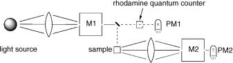
Fluorescence spectrophotometers are single-beam instruments. The basic setup of a conventional instrument with a continuous light source (usually a xenon arc) is shown in Figure 3.12. Emission spectroscopy is highly sensitive because it is basically a zerobackground technique and because photomultipliers are able to detect single photons with high probability under good operating conditions. A photoelectron released at the photocathode by a single incident photon produces an avalanche of electrons (typically >106 electrons). The quoted time resolution of photomultipliers refers to the width of a single pulse (usually about 1–2 ns), not the time elapsing between the ejection of a photoelectron at the photocathode and the arrival of the pulse at the anode. Cooling the multiplier housing can reduce thermal release of electrons. Moreover, thermal electrons usually give pulses of lower intensity. Electronic gates that suppress signals below a certain threshold can be used to suppress the background noise further. This technique is called photon counting; only the pulses that exceed a certain threshold, say 106 electrons, are counted. Fluorescence spectra are recorded by setting the monochromator M1, which selects the excitation wavelength, to an absorption maximum of the sample and scanning the monochromator M2.
In the geometric arrangement shown in Figure 3.12, the emission is collected at an angle of approximately 90 to the excitation beam (right-angle arrangement). To avoid distortions of the emission spectrum by the reabsorption of emitted light (inner filter
Figure 3.12 Basic components of a steady-state fluorescence spectrophotometer. The boxes M1 and M2 are monochromators and the detectors PM1 and PM2 are photomultipliers

88 |
Techniques and Methods |
effect), optically dilute solutions should be used. For measurements that must be done on optically dense samples, most instruments provide a front-face arrangement (the sample is irradiated at an angle of 45 and the emission is observed from the front face at an angle of about 30 to avoid reflections of the excitation beam).
Good practice in recording and correcting fluorescence spectra is mandatory and less straightforward than in absorption spectroscopy. The high sensitivity of emission spectroscopy permits the detection and quantification of extremely small amounts of luminescent compounds such as benzopyrene in industrial wastewater or in a river. Conversely, emission spectroscopy of weakly luminescent compounds is extremely sensitive to impurities with strong luminescence. Such impurities can be present in the sample or solvent, the glassware used to prepare the solution or the sample cell itself. A blank spectrum should be recorded with the pure solvent to correct for small impurity emissions and also for Rayleigh scattering and Raman emission by the solvent. Even when these trivial sources have been eliminated or at least quantified for later correction, a photoreaction of the sample that produces a fluorescent compound upon exposure to daylight or to the relatively strong excitation beam of the spectrometer can vitiate the results.
Fluorescence excitation spectra are recorded by setting the monochromator M2 to an emission maximum of the sample and scanning the excitation wavelength with the monochromator M1 (see also Special Topic 3.3). Excitation spectra are action spectraa; the emission intensity is proportional to the amount of light absorbed by the fluorescent sample at the excitation wavelength (Figure 4.23) provided that Vavilov s rule (Section 2.1.7) holds. The right-angle arrangement must be used. An excitation spectrum will faithfully reproduce the absorption spectrum of the fluorescent compound only when the intensity of the excitation beam is calibrated by the quantum counter (see below) and when the absorbance of the sample is less than 0.05 (see Section 3.9.1, Equation 3.18). At higher absorbances, the amount of light will be attenuated substantially before it reaches the central part of the sample, which is focused on to the slit of the monochromator M2.
The choice of slit widths at the monochromators is important. Small slits give better spectral resolution, while reducing the amount of light transmitted. Hence a compromise must always be made. The low light intensities associated with small slits may be compensated by increasing the sensitivity of the detector (higher voltage) and the integration times (slower scan speed). However, these will also increase the background. Whereas the slit widths at the entrance and exit of a monochromator should be the same for best performance, the slit widths at M1 and M2 can and usually should, be chosen differently. Small slit widths are chosen at M2 to improve the resolution of emission spectra, while small widths at M1 are required to achieve adequate resolution of excitation spectra. Similar arguments apply when double monochromators are used for M1 or M2.
Excitation spectra are especially useful for analysing mixtures. If the emission spectrum is (in part) due to an impurity, the excitation spectrum is likely to differ markedly from the absorption spectrum of the sample. This may be used in low-temperature work (Section 3.10) to determine whether an absorption spectrum produced by irradiation is due to a single photoproduct.
a An action spectrum is a plot of a biological, chemical or physical response per number of incident (prior to absorption) photons versus wavelength or wavenumber.

Steady-State Emission Spectra and their Correction |
89 |
Few compounds emit substantial phosphorescence in solution; biacetyl is a well-known exception to the rule. Phosphorescence lifetimes tend to be much longer (milliseconds) than fluorescence lifetimes (nanoseconds; see Section 2.1.1), so that highly purified solvents must be used and thoroughly degassed to reduce quenching by dioxygen and other adventitious
impurities. To prevent diffusional quenching, the compounds are generally dissolved in solvent mixtures157,159 that freeze to clear glasses when cooled to 77 K, such as diethyl
ether–isopentane–ethanol (5 : 5 : 2) or alkane–solvent mixtures. The sample cell (usually a quartz tube) is dipped into liquid nitrogen contained in a transparent quartz Dewar vessel.
Alternatively, glassy solutions that are solid at room temperature [borax or poly(methyl methacrylate, PMMA) glass] can be used for phosphorescence measurements of organic and inorganic solutes. Freshly distilled methyl methacrylate solutions are polymerized in stoppered glass tubes by warming at 80 C for a few days. The resulting mould is readily cut to any desired shape and polished to produce transparent blocks. Oxygen is mostly consumed during the polymerization and the diffusion of air into the moulds is fairly slow (<1 mm per month); such samples can be used as reference samples to set up a phosphorescence spectrometer or for classroom demonstration of the slow phosphorescence decay of naphthalene, for example, which lasts for many seconds.
Phosphorescence spectra are commonly weaker than fluorescence spectra, even when solid sample solutions are probed. For unperturbed detection of phosphorescence, the fluorescence must, therefore, be eliminated. This is readily achieved by surrounding the sample with a metal cylinder that is rotated at variable speed by a motor ( rotating can ). A hole in the cylinder exposes the sample to the excitation beam for a short period, during which the detector does not see the sample. Rotation of the can subsequently opens the sample to the detector, long after the fluorescence has decayed. The phosphorescence lifetime can then be determined from the intensity dependence of the phosphorescence on the rotational speed. In modern instruments, the elimination of fluorescence is commonly achieved by replacing the continuous light source with a pulsed source (a stroboscope or a pulsed laser) and the photomultiplier is electronically deactivated during and shortly after the excitation pulse.
Special Topic 3.3: Phosphorescence excitation spectra
Singlet–triplet absorption spectra are very difficult to measure, because the absorption coefficients for these forbidden transitions are extremely weak in organic molecules. In principle, one could resort to using very high concentrations and pathlengths, but in practice this requires materials of extremely high purity and the method fails at shorter excitation wavelengths where singlet–singlet absorption sets in. Few reliable results have been obtained in this way with organic compounds (for an example, see Figure 6.15).
The intensity of singlet–triplet absorption can be increased by using heavy-atom media (CBr4 or liquid xenon) and particularly by paramagnetic enhancement under high pressures of dioxygen (oxygen pressure method). Most of these measurements were done by Evans around 1960 using oxygen pressures up to 130 atm. To put reactive organic molecules and solvents under high oxygen pressure is, however, a dangerous venture. Evans reported: Only one measurement was made on an acetylene–oxygen mixture at high pressures (acetylene 20 atm, oxygen 100 atm). When the needle valve

90 |
Techniques and Methods |
was opened to release the pressure, a violent explosion occurred which reduced the quartz windows of the cell to fine dust and blew off the stainless steel end-plates at high velocity. 178
The more convenient method of phosphorescence excitation was introduced by Kearns in 1965. Because emission spectroscopy is much more sensitive than absorption, particularly for phosphorescence that can efficiently be separated from stray light and fluorescence, the determination of singlet–triplet absorption spectra by monitoring the resulting phosphorescence emission has often been successful with comparatively little effort.
Because fluorescence spectrometers are single-beam instruments, a number of corrections are required to obtain reproducible and meaningful emission spectra. Temporal fluctuations of the light source, and also the variations of its intensity at different excitation wavelengths, are corrected by means of a quantum counter that consists of a triangular cell containing a solution of a fluorescent dye and a photomultiplier, which constantly monitors the total fluorescence emission from that cell (PM1, Figure 3.12). The fluorescent dye, usually Rhodamine 6G, must be sufficiently concentrated to absorb the incident light completely at all wavelengths of excitation l and it must have a fluorescence quantum yield that is independent of l. The signal from PM1 is then proportional to the number of photons per unit time in the excitation beam, part of which is focused on to the quantum counter cell. Fluctuations of the intensity of the light source in time, and also its variations at different excitation wavelengths when scanning monochromator M1 to record excitation spectra, are automatically corrected by dividing the output signal of the fluorescence detector PM2 by that of PM1 (ratiometric measurement). Obviously, the correction of excitation spectra works only up to the red edge of the absorption by the fluorescent dye.
Current spectrometers use a grating, so that the spectral dispersion is linear in wavelength and the spectral bandpass (the width dl of light from a white source passing the monochromator) is independent of wavelength. Therefore, spectrofluorimeters generally plot spectra on a wavelength scale. If an emission spectrum is converted to a wavenumber scale, it is essential to convert the instrument readings, the emitted spectral radiant power per wavelength interval Plem according to Pn~ ¼ Pl=n~2 (see footnote to Equation 2.3), which results in substantial changes of the spectral shape. For the determination of fluorescence quantum yields (Section 3.9.5) or of F€orster overlap integrals (Section 2.2.2), it is unnecessary, and therefore not recommended, to convert spectra from a wavelength to a wavenumber scale.
Correction of emission spectra is required, because the transmission efficiency of the monochromators and particularly the sensitivity of the detectors depend on the wavelength and the polarization of the emitted light. A magic-angle arrangement of polarizers may be used to avoid distortions due to polarized emission from solid samples.175 Commercial instruments may be delivered with a sensitivity function S(l) that allows correction of the recorded emission spectra by multiplication with the recorded signal, Plem ¼ PlobsSðlÞ. However, the function S(l) usually changes substantially as the instrument ages, so it should be calibrated at regular intervals. This can be done either using standard fluorescent dyes179 such as quinine sulfate, the true emission spectra of which have been determined accurately,
Time-Resolved Luminescence |
91 |
or with a calibrated tungsten lamp. For the conversion of an emission spectrum to a wavenumber scale, the sensitivity function S(l) must be replaced by S(n~) (Equation 3.2).
Sðn~Þ ¼ SðlÞjdl=dn~j ¼ SðlÞ=n~2
Equation 3.2
3.5 Time-Resolved Luminescence
Recommended reviews.177,180 See also Section 3.13.
Recent developments of pulsed light sources, optical components, fast and sensitive detectors and electronic equipment for data collection and analysis have permitted the construction of numerous instruments, often commercially available, for the collection of luminescence data with excellent resolution in time, spectral distribution and space. The sensitivity has reached the ultimate level that allows the characterization of such properties for single molecules (see Section 3.13). Only an overview of some of these techniques is given here.
In pulse fluorimetry, the sample is excited by a short pulse of light from a laser or from a spark gap (similar to the spark gaps used to ignite combustion in motor engines). Spark gaps are inexpensive and produce highly reproducible excitation pulses of about 2 ns width. Spark gap instruments are operated at repetition rates of 104–105 Hz and the fluorescence signals are accumulated using single photon counting (Section 3.4) and an electronic time-to-amplitude converter. If the duration of the pulse is comparable to or longer than the lifetime of the fluorescence decay, as is often the case, the fluorescence intensity rises in time with the excitation pulse, passes through a maximum and reflects the true decay function of the sample only when the intensity of the pulse becomes negligible. However, the excellent statistics of the averaged signal permit a mathematical deconvolution of the decay signal from the excitation pulse shape. In this way, a time resolution of about 200 ps can be achieved for fluorescence lifetimes. This can be improved by an order of magnitude by using short excitation pulses from mode-locked lasers and fast microchannel plate photomultipliers as detectors (Section 3.1).
In phase-modulation fluorimeters, a continuous excitation beam is modulated at a gigahertz frequency using a Pockels cell and the fluorescence signal is detected with a lock-in amplifier. Time resolutions achievable depend on the instrumentation and are comparable to those in pulse fluorimetry. Streak cameras (Section 3.1) offer the muliplexer advantage of recording the time evolution of complete emission spectra. The time resolution reaches a few picoseconds on the fastest instruments. However, signal averaging is usually required to achieve an adequate signal-to-noise ratio and jitter of the trigger signal may then blur the accumulated signal on the time axis.
Ultrashort fluorescence lifetimes are best determined by photon upconversion. An excellent description of the technique for non-specialists wishing to set up an experiment is in preparation as part of a current IUPAC project on ultrafast intense laser chemistry .181 The time resolution is basically limited by the temporal width of the laser pulses that are being used. An intense gate pulse at frequency nG is mixed with the fluorescence at a frequency nF in a nonlinear optical crystal (Special Topic 3.1), to create a short pulse at the sum frequency nU. The gate pulse thus represents a time window for the fluorescence
92 |
Techniques and Methods |
during which the latter is upconverted and the intensity of the upconverted light is measured. By controlling the optical delay between the fluorescence and the gating pulse, kinetic traces of the fluorescence can be obtained. Because the upconverted signal appears far to the blue of the fluorescence band, it is easily separated from the signals at frequencies nG and nF by a monochromator or an optical filter.
3.6 Absorption and Emission Spectroscopy with Polarized Light
Recommended textbook.182
The orientation of transition moments in the molecular framework can be predicted by quantum mechanical calculations (Sections 2.1.4 and 4.4). Experimentally, the direction of transition moments can be assessed by studying the absorption of linearly polarized light by samples in which the molecules are preferentially oriented. Complete orientation is available in single crystals. However, optical measurements on single crystals are demanding and rarely practicable, not least because extremely thin crystals are required for absorption studies.
Partial orientation is much easier to achieve and generally sufficient to determine the direction of the transition moments, particularly with respect to any axes of symmetry that the molecules may have. Partial orientation can be achieved by photoselection using a linearly polarized excitation source, by application of an electric field or by dissolving the solute in a transparent anisotropic medium (liquid crystals, stretched polymers).182 Photoselection is the basis of emission anisotropy measurements discussed below. It is also used for molecules that can be either generated or destroyed photochemically in a rigid medium such as poly(methyl methacrylate) or glassy solvents at low temperature. Preferential alignments of dipolar molecules that are achievable by electrostatic fields are unfortunately fairly small.
By far the simplest method for the preparation of partially oriented samples is the doping
of stretched polyethylene sheets, which was developed by Thulstrup, Eggers and Michl.182,183 It can be applied in any laboratory and requires no special equipment
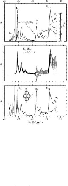
other than a UV–VIS or IR spectrometer and linear polarizers. Commercial polyethylene usually contains various additives such as UV stabilizers, which must be removed by extraction, but optically clean sheets are available. The sheets are doped either by swelling them in a solution of the probe and evaporating the solvent or by keeping them under vacuum under vapours of the substrate. The sheets are then stretched to about six times their original length and their absorption spectrum is recorded twice with linearly polarized light beams with the electric vector parallel and perpendicular to the stretching direction. An example taken from the literature 182 is shown in Figure 3.13. A series of linear combinations of the two spectra is generated by computer (centre diagram in Figure 3.13), two of which are chosen such that some spectral features disappear from one or the other of the two combinations. Cooling of the sample in the spectrometer improves the resolution, but is not required. It is well established that the above procedure for spectral reduction reliably recovers the polarized spectra of molecules with a plane of symmetry just as they would be obtained with a fully oriented sample. For details of the procedure and analysis of polarized spectra of partially oriented samples, the reader is referred to the original literature.
Absorption and Emission Spectroscopy with Polarized Light |
93 |
Figure 3.13 Pyrene in stretched polyethylene at 77 K. Top: baseline-corrected polarized absorption spectra EZ (parallel) and EY (perpendicular to the stretching direction). Centre: linear combinations of the polarized spectra EZ and EY. Bottom: reduced UV spectra of pyrene. Az ¼ EZ 1.0EY and AY ¼ 1.75(EY 0.36EZ). Adapted by permission from ref. 182. The Platt symbols Lb, La, Bb and Ba labelling the electronic transitions are explained in Section 4.7. The polarization of the weak Lb band shown on the left (<29 000 cm 1, spectra recorded at higher concentration) is of mixed polarization
Most light sources, lasers in particular, are linearly polarized to some degree. As a result, the emission from the sample may also be polarized. The degree of anisotropy R is defined by Equation 3.3:
R |
III I? |
; |
|
0:2 R 0:4 |
|
¼ III þ 2I? |
|
||
Equation 3.3 Degree of emission anisotropy
where I|| and I? are the radiant intensities measured with the linear polarizer for emission parallel and perpendicular, respectively, to the electric vector of linearly polarized incident
94 Techniques and Methods
electromagnetic radiation. The quantity I|| þ 2I? is proportional to the total emission intensity.
In an isotropic sample with randomly oriented chromophores, the emission anisotropy arises from preferential excitation (photoselection) of those molecules that happen to be oriented such that their transition moment of absorption is oriented parallel to the polarization of the exciting light. The theoretical values of R depend on the angle f between the transition moments of absorption and emission, ma and me: R ¼ h3cos2f 1i/5, where hi denotes an average over the orientations of the photoselected molecules. This leads to the range of values given in Equation 3.3, that is, 1/5 for f ¼ 90 and 2/5 for f ¼ 0 . In practice, R is often reduced by (a combination of) the following depolarizing events: rotational diffusion of the emitter during its lifetime, overlap of differently polarized transitions in the range of excitation or emission wavelengths measured, energy transfer between the emitting chromophores (Section 2.2.2) and adiabatic reactions of the emitter such as proton transfer (Section 5.3). Time-resolved measurements of anisotropy can be used to determine the rate of rotational diffusion of large molecules such as tagged biopolymers, when the rotational time constant is comparable to the lifetime of emission. Rotational diffusion can be reduced or suppressed in highly viscous media.
3.7 Flash Photolysis
Recommended reviews are mentioned in the second paragraph below.
Since its invention by Norrish and Porter in 1949,184 flash photolysis is the most important tool to produce transient intermediates in sufficient concentration for time-resolved spectroscopic detection and for the identification of elementary reaction steps (see Section 5.1). The term photolysis strictly implies the light-induced breaking of chemical bonds (the Greek expression lysis means dissolution or decomposition). However, since its inception, the term flash photolysis has been used to describe the technique of excitation by short pulses of light, irrespective of the processes that follow.
Transient intermediates are most commonly observed by their absorption (transient absorption spectroscopy; see ref. 185 for a compilation of absorption spectra of transient species). Various other methods for creating detectable amounts of reactive intermediates such as stopped flow, pulse radiolysis, temperature or pressure jump have been invented and novel, more informative, techniques for the detection and identification of reactive intermediates have been added, in particular EPR, IR and Raman spectroscopy (Section 3.8), mass spectrometry, electron microscopy and X-ray diffraction. The technique used for detection need not be fast, provided that the time of signal creation can be determined accurately (see Section 3.7.3). For example, the separation of ions in a mass spectrometer (time of flight) or electrons in an electron microscope may require
microseconds or longer. Nevertheless, femtosecond time resolution has been achieved,186,187 because the ions or electrons are formed by a pulse of femtosecond
duration (1 fs ¼ 10 15 s). Several reports with recommended procedures for nanosecond flash photolysis,137,188–191 ultrafast electron diffraction and microscopy,192 crystal-
lography193 and pump–probe absorption spectroscopy194,195 are available and a general treatise on ultrafast intense laser chemistry is in preparation by IUPAC.